Chapter 8 Major Earthquake Analysis

We apply the concepts in the previous chapters to the series of annual counts of major earthquakes (i.e. magnitude 7 and above) from the textbook.

The data can be read into R

eq_dat <- read.table("http://www.hmms-for-time-series.de/second/data/earthquakes.txt")

We use the following packages for the analysis

# Load packages
library(kableExtra)
library(tidyverse)
library(gridExtra)
library(momentuHMM)
library(rstan)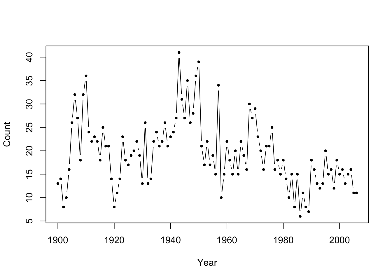

Figure 8.1: Number of major earthquakes worldwide from 1900-2006.

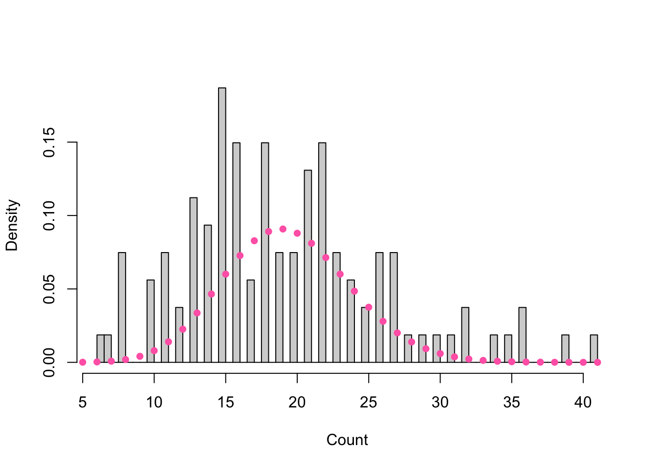
Figure 8.2: Histogram of major earthquakes overlaid with a Poisson density of mean equal to the observed counts.

Table 8.1: Summary of the major earthquakes.

mean	variance
19.36	51.57

Fitting a Poisson Mixture Distribution

Note: See Preliminaries

We may consider fitting a Poisson mixture distribution since earthquake counts are unbounded and there appears to be overdispersion as evident by the multimodal peaks in Figure 8.2 and sample variance \(s^2 \approx 52 > 19 \approx \bar{x}\) in Table 8.1.

Suppose \(m=3\) and the three components are Poisson-distributed with means \(\lambda_1, \lambda_2\), and \(\lambda_3\). Let \(\delta_1\), \(\delta_2\), and \(\delta_3\) be the respective mixing parameters. The mixture distribution \(p\) is given by

\[p(x) = \delta_1 \frac{\lambda_1^x e^{-\lambda_1}}{x!} + \delta_2 \frac{\lambda_2^x e^{-\lambda_2}}{x!} + \delta_3 \frac{\lambda_3^x e^{-\lambda_3}}{x!}\]

The likelihood is given by

\[L(\lambda_1, \lambda_2, \lambda_3, \delta_1, \delta_2|x_1, \dots, x_n) = \prod_{i=1}^n \left( \delta_1 \frac{\lambda_1^{x_i} e^{-\lambda_1}}{x_i!} + \delta_2 \frac{\lambda_2^{x_i} e^{-\lambda_2}}{x_i!} + (1 - \delta_1 - \delta_2) \frac{\lambda_3^{x_i} e^{-\lambda_3}}{x_i!} \right)\]

The log-likelihood can be maximized using the unconstrained optimizer nlm on reparameterized parameters by the following:

Step 1: Reparameterize the “natural parameters” \(\boldsymbol{\delta}\) and \(\boldsymbol{\lambda}\) into “working parameters” \(\eta_i = \log \lambda_i \qquad{(i = 1, \dots, m)}\) and \(\tau_i = \log \left(\frac{\delta_i}{1 - \sum_{j=2}^m \delta_j}\right) (i = 2, \dots, m)\)

n2w <- function(lambda, delta)log(c(lambda, delta[-1]/(1-sum(delta[-1]))))

Step 2: Compute the negative log-likelihood using the working parameters

mllk <- function(wpar, x){
  zzz <- w2n(wpar)
  -sum(log(outer(x, zzz$lambda, dpois)%*%zzz$delta))}

Step 3: Transform the parameters back into natural parameters

w2n <- function(wpar){
  m <- (length(wpar)+1)/2
  lambda <- exp(wpar[1:m])
  delta <- exp(c(0, wpar[(m+1):(2*m-1)]))
  return(list(lambda=lambda, delta=delta/sum(delta)))}

Hence, for a Poisson mixture distribution with means \(\lambda_1, = 10, \lambda_2 = 20, \lambda_3 = 25\) and probabilities \(\delta_1 = \delta_2 = \delta_3 = \frac{1}{3}\),

wpar <- n2w(c(10, 20, 25), c(1,1,1)/3)

w2n(nlm(mllk, wpar, eq_dat$Count)$estimate)

we obtain the following parameter estimates

Table 8.2: Parameter estimates for the fitted three component Poisson independent mixture model.

lambda	delta
12.73573	0.2775329
19.78515	0.5928037
31.62940	0.1296634

and the negative log likelihood

nlm(mllk, wpar, eq_dat$Count)$minimum

## [1] 356.8489

Note: See Table 1.2 and Figure 1.4 of the textbook for a comparison of fitted mixture models with varying number of components.

Fitting a Poisson-HMM by Numerical Maximization

Note: See Introduction to Hidden Markov Models and Appendix A of the textbook.

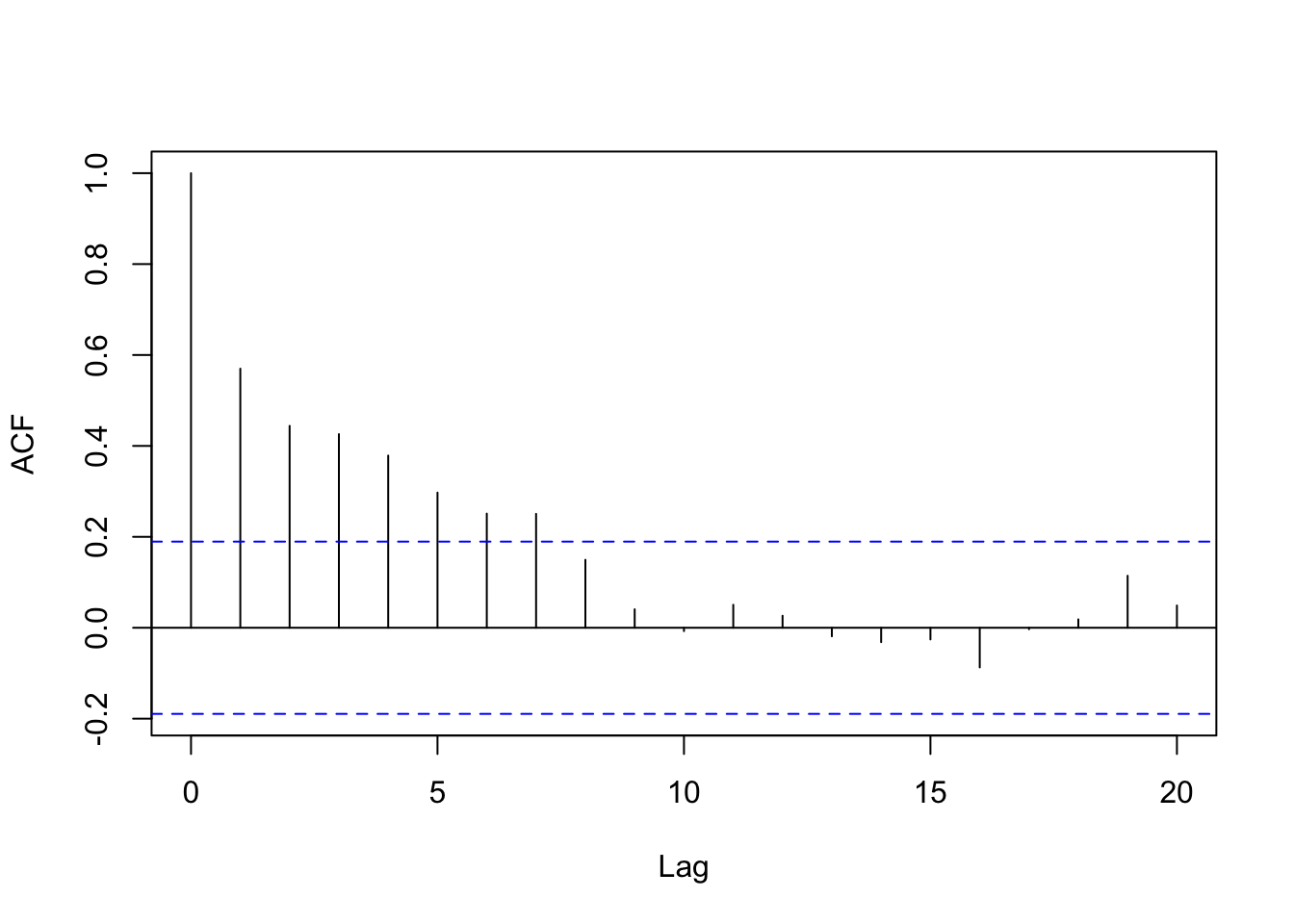
Figure 8.3: Autocorrelation plot for major earthquakes.

Instead of fitting an (independent) Poisson mixture distribution, we may consider fitting a Poisson-HMM to account for the strong, positive serial dependence as evident in Figure 8.3.

Step 1: Reparameterize the “natural parameters” \(\boldsymbol{\Gamma}, \boldsymbol{\lambda}\), and \(\boldsymbol{\delta}\) to the “working parameters”.

Set \[\eta_i = \log \lambda_i \qquad{(i = 1, \dots, m)}\]

\[\nu_{ij} = \begin{cases} 1 & \qquad{\text{for } i = j} \\ \log(\gamma_{ij}) & \qquad{\text{for } i \neq j} \end{cases}\]

\[\delta_i = \begin{cases} \log \left(\frac{(\delta_2, \dots, \delta_m)}{\delta_1}\right) & \qquad{\text{if not stationary}}\\ \text{NULL} & \qquad{\text{otherwise}} \end{cases}\]

See Reparameterization to Avoid Constraints.

pois.HMM.pn2pw <- function(m,lambda,gamma,delta=NULL,stationary=TRUE){ 
  
  # eta = log(lambda)
  tlambda <- log(lambda)
  if(m==1) return(tlambda)
 
  # For i = j, nu_ii = 1 
  foo     <- log(gamma/diag(gamma))
  
  # For i != j, nu_ij = log(gamma_ij)
  tgamma  <- as.vector(foo[!diag(m)])
  
  # If stationary, set to pi = null
  if(stationary) {tdelta  <- NULL}
  # Otherwise, pi = log((delta_2, ..., delta_m)/delta_1)
    else {tdelta <- log(delta[-1]/delta[1])}
 
  parvect <- c(tlambda,tgamma,tdelta)
  return(parvect)
}

Note: pois.HMM.pn2pw takes in arguments m number of states (numeric), lambda Poisson means (vector), delta initial probabilities, and stationary (TRUE/FALSE). By default, the MC is assumed to be stationary with the initial distribution equal to the stationary distribution. The function returns a vector containing the working parameters.

Step 2: Compute the log-likelihood by the forward algorithm using the scaling strategy.

The general algorithm is:

\(w_1 \leftarrow \boldsymbol{\delta P} (x_1) \boldsymbol{1'};\) \(\boldsymbol{\phi}_1 \leftarrow \boldsymbol{\delta P} (x_1);\) \(l \leftarrow \log w_1\)

for \(t=2, 3, \dots, T\)

\[\begin{align} \boldsymbol{v} &\leftarrow \boldsymbol{\phi}_{t-1} \boldsymbol{\Gamma P} (x_t)\\ u & \leftarrow \boldsymbol{v 1'}\\ l &\leftarrow l + \log u\\ \boldsymbol{\phi}_t & \leftarrow \frac{\boldsymbol{v}}{u} \end{align}\]

See Scaling the Likelihood Computation and Note (4).

pois.HMM.lforward <- function(x,mod){
  
  n             <- length(x)
  lalpha        <- matrix(NA,mod$m,n)
  
  # At time t=1
  foo           <- mod$delta*dpois(x[1],mod$lambda)
  sumfoo        <- sum(foo)
  lscale        <- log(sumfoo)
  foo           <- foo/sumfoo
  
  lalpha[,1]    <- lscale+log(foo)
  
  # For t > 1
  for (i in 2:n){
    foo          <- foo%*%mod$gamma*dpois(x[i],mod$lambda)
    sumfoo       <- sum(foo)
    lscale       <- lscale+log(sumfoo)
    foo          <- foo/sumfoo
    lalpha[,i]   <- log(foo)+lscale
    }
  return(lalpha)
}

Note: pois.HMM.lforward takes in arguments x data and mod list consisting of m states, lambda means for the Poisson state-dependent distribution, and delta initial probabilities.

Step 3: Maximize the log-likelihood/Minimize the negative log-likelihood

The function nlm in R performs the minimization of any function using a Newton-type algorithm. In order to minimize the negative log-likelihood, we first write a function that compute the negative log-likelihood from the working parameters. The same forward algorithm scheme applies.

pois.HMM.mllk <- function(parvect,x,m,stationary=TRUE,...)
{
 if(m==1) return(-sum(dpois(x,exp(parvect),log=TRUE)))
 n        <- length(x)
 pn       <- pois.HMM.pw2pn(m,parvect,stationary=stationary)
 foo      <- pn$delta*dpois(x[1],pn$lambda)
 sumfoo   <- sum(foo)
 lscale   <- log(sumfoo)
 foo      <- foo/sumfoo
 for (i in 2:n)
   {
   if(!is.na(x[i])){P<-dpois(x[i],pn$lambda)}
     else {P<-rep(1,m)}
   foo    <- foo %*% pn$gamma*P
   sumfoo <- sum(foo)
   lscale <- lscale+log(sumfoo)
   foo    <- foo/sumfoo
   }
 mllk     <- -lscale
 return(mllk)
}

Step 4: Transform the parameters back into natural parameters.

Set

\[\hat{\lambda_i} = \exp(\hat{\eta_i}) \qquad{(i = 1, \dots, m)}\]

\[\hat{\gamma}_{ij} = \frac{\exp(\hat{\nu_{ik}})}{\sum_{k=1, k \neq i}^m\exp(\hat{\nu_ik})} \qquad{\text{for } (i, j = 1, \dots, m)}\]

\[\hat{\boldsymbol{\delta}} = \begin{cases} \boldsymbol{1} (\boldsymbol{I} - \hat{\boldsymbol{\Gamma}} + \boldsymbol{U})^{-1}& \qquad{\text{if stationary}}\\ \frac{(1, \exp(\hat{\delta_2}), \dots, \exp(\hat{\delta}_m))}{1 + \exp(\hat{\delta_2}) + \dots + \exp(\hat{\delta}_m)} & \qquad{\text{otherwise}} \end{cases}\]

pois.HMM.pw2pn <- function(m,parvect,stationary=TRUE){
 lambda        <- exp(parvect[1:m])
 gamma         <- diag(m)
 if (m==1) return(list(lambda=lambda,gamma=gamma,delta=1))
 gamma[!gamma] <- exp(parvect[(m+1):(m*m)])
 gamma         <- gamma/apply(gamma,1,sum)
 if(stationary){delta<-solve(t(diag(m)-gamma+1),rep(1,m))}
   else {foo<-c(1,exp(parvect[(m*m+1):(m*m+m-1)]))
   delta<-foo/sum(foo)}
 return(list(lambda=lambda,gamma=gamma,delta=delta))
}

Note: pois.HMM.pw2pn takes in arguments m number of states, parvect working parameters (vector), and stationary (TRUE/FALSE). By default, the MC is assumed to be stationary with the initial distribution equal to the stationary distribution. The function returns a list containing the natural parameters.

We can combine the parts above into the pois.HMM.mle function.

pois.HMM.mle <- function(x,m,lambda0,gamma0,delta0=NULL,stationary=TRUE,...){
 parvect0  <- pois.HMM.pn2pw(m,lambda0,gamma0,delta0,stationary=stationary)
 mod       <- nlm(pois.HMM.mllk,parvect0,x=x,m=m,stationary=stationary)
 pn        <- pois.HMM.pw2pn(m=m,mod$estimate,stationary=stationary)
 mllk      <- mod$minimum
 np        <- length(parvect0)
 AIC       <- 2*(mllk+np)
 n         <- sum(!is.na(x))
 BIC       <- 2*mllk+np*log(n)
 list(m=m,lambda=pn$lambda,gamma=pn$gamma,delta=pn$delta,code=mod$code,mllk=mllk,AIC=AIC,BIC=BIC)
}

Hence, for a three-state Poisson-HMM with the following parameters

\[\boldsymbol{\lambda} = (10, 20, 25)\]

\[\boldsymbol{\Gamma} = \begin{pmatrix} 0.8 & 0.1 & 0.1\\ 0.1 & 0.8 & 0.1\\ 0.1 & 0.1 & 0.8 \end{pmatrix}\]

m = 3
lambda = c(10, 20, 25)
gamma = matrix(c(0.8,0.1,0.1,0.1,0.8,0.1,0.1,0.1,0.8),3,3,byrow=TRUE)

if we assume that the MC is stationary

eq_init_s <- list(m=m,
            lambda=lambda,
            gamma = gamma)

(mod3s<-pois.HMM.mle(eq_dat$Count, eq_init_s$m,eq_init_s$lambda,eq_init_s$gamma,stationary=TRUE))

## $m
## [1] 3
## 
## $lambda
## [1] 13.14573 19.72101 29.71437
## 
## $gamma
##              [,1]      [,2]       [,3]
## [1,] 9.546243e-01 0.0244426 0.02093313
## [2,] 4.976679e-02 0.8993673 0.05086592
## [3,] 1.504495e-09 0.1966420 0.80335799
## 
## $delta
## [1] 0.4436420 0.4044983 0.1518597
## 
## $code
## [1] 1
## 
## $mllk
## [1] 329.4603
## 
## $AIC
## [1] 676.9206
## 
## $BIC
## [1] 700.976

and if we do not assume stationary and that \(\boldsymbol{\delta} = (\frac{1}{3}, \frac{1}{3}, \frac{1}{3})\) and that the initial distribution is \(\boldsymbol{\delta} = (\frac{1}{3}, \frac{1}{3}, \frac{1}{3})\)

eq_init_ns <- list(m=m,
            lambda=lambda,
            gamma = gamma,
            delta = rep(1, m)/m)

(mod3h <- pois.HMM.mle(eq_dat$Count,eq_init_ns$m,eq_init_ns$lambda,eq_init_ns$gamma,delta=eq_init_ns$delta,stationary=FALSE))

## $m
## [1] 3
## 
## $lambda
## [1] 13.13374 19.71312 29.70964
## 
## $gamma
##              [,1]       [,2]       [,3]
## [1,] 9.392937e-01 0.03209754 0.02860881
## [2,] 4.040106e-02 0.90643731 0.05316163
## [3,] 9.052023e-12 0.19025401 0.80974599
## 
## $delta
## [1] 9.999998e-01 8.700482e-08 8.281945e-08
## 
## $code
## [1] 1
## 
## $mllk
## [1] 328.5275
## 
## $AIC
## [1] 679.055
## 
## $BIC
## [1] 708.4561

Parametric Bootstrapping for Confidence Intervals

We can also perform parameteric bootstrapping to obtain confidence intervals of the above estimates.

Note: See Obtaining Standard Errors and Confidence Intervals.

Step 1: Fit the model

eq_mle <- pois.HMM.mle(eq_dat$Count,eq_init_ns$m,eq_init_ns$lambda,eq_init_ns$gamma,delta=eq_init_ns$delta,stationary=FALSE)

Step 2: Generate a bootstrap sample from the fitted model.

The following function generates a sample from a Poisson-HMM of length ny from starting values m number of states, lambda means for the Poisson state-dependent distribution, and delta initial probabilities which are stored as mod (list).

pois.HMM.generate_sample  <- function(ny,mod){
 mvect                    <- 1:mod$m
 state                    <- numeric(ny)
 state[1]                 <- sample(mvect,1,prob=mod$delta)
 for (i in 2:ny) state[i] <- sample(mvect,1,prob=mod$gamma[state[i-1],])
 x                        <- rpois(ny,lambda=mod$lambda[state])
 return(x)
}

boot_sample <- pois.HMM.generate_sample(length(eq_dat$Count), eq_mle)

Step 3: Estimate parameters using the bootstrap sample.

boot_mle <- pois.HMM.mle(boot_sample, eq_mle$m, eq_mle$lambda, eq_mle$gamma)

## Warning in nlm(pois.HMM.mllk, parvect0, x = x, m = m, stationary = stationary):
## NA/Inf replaced by maximum positive value

Step 4: Repeat (for a large) B times.

We can combine the parts above into the pois.HMM.boot function.

pois.HMM.boot <- function(B, x, m, lambda0, gamma0, delta0=NULL, stationary=TRUE){
  
  # Fit the model
  mod <- pois.HMM.mle(x, m, lambda0, gamma0, stationary=stationary)
  
  # Initialize
  bs_sample <- list()
  bs_mod <- list()
  
  # Generate B bootstrap samples
  for(i in 1:B){
    a = TRUE
    while(a){
      tryCatch({
        set.seed(i)
        bs_sample[[i]] <- pois.HMM.generate_sample(length(x), mod)
        bs_mod[[i]] <- pois.HMM.mle(bs_sample[[i]], m, mod$lambda, mod$gamma, mod$delta)
        a = FALSE
        },
        error=function(w){
          a = TRUE
        })
    }
    }
  return(bs_mod)
}

Note: Some errors would occasionally arise from solving the stationary distribution of bootstrap samples that may not have had a unique stationary distribution. To overcome this, the tryCatch function was used to throw out these problematic samples and regenerate a new sample. As there were at most two samples that resulted in the error, the generated bootstrap samples should still be representative of the dataset.

Hence, for the three-state Poisson-HMM with parameters

\[\boldsymbol{\lambda} = (10, 20, 25)\]

\[\boldsymbol{\Gamma} = \begin{pmatrix} 0.8 & 0.1 & 0.1\\ 0.1 & 0.8 & 0.1\\ 0.1 & 0.1 & 0.8 \end{pmatrix}\]

\[\boldsymbol{\delta} = (\frac{1}{3}, \frac{1}{3}, \frac{1}{3})\]

eq_boot <- pois.HMM.boot(500, eq_dat$Count, eq_init_ns$m, eq_init_ns$lambda, eq_init_ns$gamma, delta=eq_init_ns$delta)

and the \(90\%\) confidence interval using the “percentile method”

# Create dataframe for parameters from bootstrap samples
eq_lambda_boot <- sapply(eq_boot, "[[", 2)
eq_lambda_boot <- t(eq_lambda_boot)
eq_lambda_boot <- as.data.frame(eq_lambda_boot)

eq_gamma_boot <- sapply(eq_boot, "[[", 3)
eq_gamma_boot <- t(eq_gamma_boot)
eq_gamma_boot <- as.data.frame(eq_gamma_boot)

eq_delta_boot <- sapply(eq_boot, "[[", 4)
eq_delta_boot <- t(eq_delta_boot)
eq_delta_boot <- as.data.frame(eq_delta_boot)

# Obtain the 90% confidence interval
eq_boot_df <- t(cbind(sapply(eq_lambda_boot, quantile, probs=c(0.05, 0.95)),
                           sapply(eq_gamma_boot, quantile, probs=c(0.05, 0.95)),
                           sapply(eq_delta_boot, quantile, probs=c(0.05, 0.95)))) %>% 
  as.data.frame() 

rownames(eq_boot_df)[1:3] <- paste0("lambda", 1:3)
rownames(eq_boot_df)[4:6] <- paste0("gamma", 1, 1:3)
rownames(eq_boot_df)[7:9] <- paste0("gamma", 2, 1:3)
rownames(eq_boot_df)[10:12] <- paste0("gamma", 3, 1:3)
rownames(eq_boot_df)[13:15] <- paste0("delta", 1:3)


eq_boot_df %>%
  round(4) %>%
  kbl(caption="Bootstrap 90% Confidence Intervals for the parameters of the three-state HMM.") %>%
  kable_minimal(full_width=T)

Table 8.3: Bootstrap 90% Confidence Intervals for the parameters of the three-state HMM.

	5%	95%
lambda1	11.8405	14.6116
lambda2	16.9308	22.0249
lambda3	19.4806	33.0097
gamma11	0.8232	0.9880
gamma12	0.0137	0.2132
gamma13	0.0000	0.0000
gamma21	0.0000	0.1162
gamma22	0.6603	0.9637
gamma23	0.0515	0.5534
gamma31	0.0000	0.1108
gamma32	0.0000	0.1908
gamma33	0.4466	0.9485
delta1	0.1370	0.7485
delta2	0.1114	0.6606
delta3	0.0404	0.3770

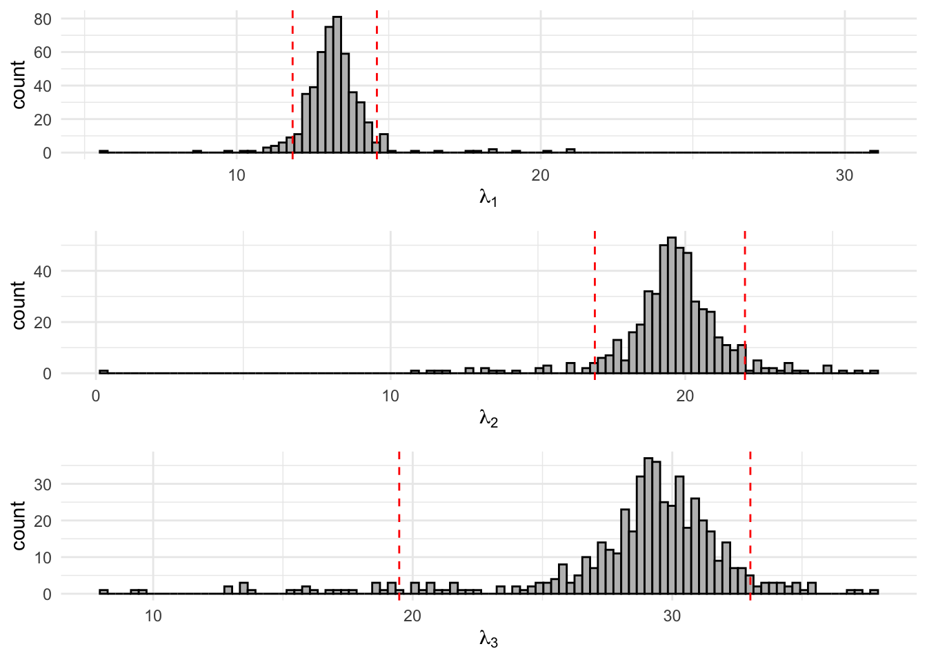
Figure 8.4: 500 Bootstrap samples for the state-dependent parameters of the fitted three-state Poisson-HMM. The area within the red dotted lines correspond to the 90% confidence interval.

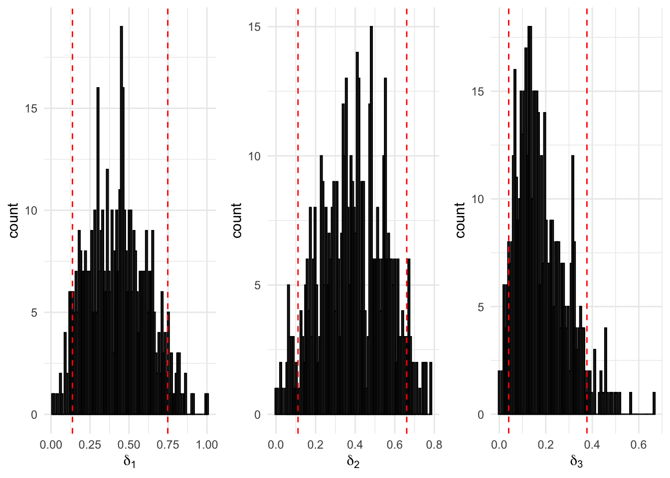
Figure 8.5: 500 Bootstrap samples for the initial probabilities of the fitted three-state Poisson-HMM. The area within the red dotted lines correspond to the 90% confidence interval.

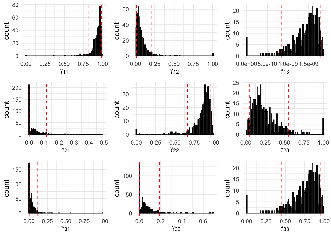
Figure 8.6: 500 Bootstrap samples for the transition probabilities of the fitted three-state Poisson-HMM. The area within the red dotted lines correspond to the 90% confidence interval.

Using momentuHMM

We can also fit the three-state Poisson-HMM from the above using momentuHMM, which is a popular package for the maximum likelihood analysis of animal movement behaviour using multivariate Hidden Markov Models. McClintock and Michelot (2018)

First, convert the data into the prepData object and set the names of the states. Since

# prepData
eq_prepped <- prepData(eq_dat,
                       coordNames = NULL,
                       covNames =  c("Count"))

# Name the states
stateNames <- c("state1", "state2", "state3")

Next, specify the state-dependent model. In our case, we fit the intercept only model.

# Fit intercept only model
formula = ~ 1

Now, fit the model using fitHMM

mod3h_momentuHMM <- fitHMM(eq_prepped, 
               nbStates=3, 
               dist=list(Count="pois"),
               Par0 = list(Count = eq_init_ns$lambda, delta=eq_init_ns$delta),
               formula = formula,
               stateNames = stateNames,
               stationary = FALSE)

The resulting MLEs are very similar to that obtained from running the functions from above.

mod3h_momentuHMM 

## Value of the maximum log-likelihood: -328.5884 
## 
## 
## Count parameters:
## -----------------
##          state1   state2   state3
## lambda 13.13513 19.70822 29.70794
## 
## Regression coeffs for the transition probabilities:
## ---------------------------------------------------
##               1 -> 2    1 -> 3    2 -> 1   2 -> 3    3 -> 1    3 -> 2
## (Intercept) -3.42222 -3.520977 -3.119039 -2.83615 -28.60659 -1.448253
## 
## Transition probability matrix:
## ------------------------------
##              state1     state2     state3
## state1 9.414330e-01 0.03072828 0.02783867
## state2 4.007763e-02 0.90674107 0.05318130
## state3 3.052488e-13 0.19027062 0.80972938
## 
## Initial distribution:
## ---------------------
##       state1       state2       state3 
## 1.000000e+00 1.833456e-08 1.427794e-08

The corresponding \(95 \%\) confidence intervals are

CIreal(mod3h_momentuHMM)

## $Count
## $Count$est
##          state1   state2   state3
## lambda 13.13513 19.70822 29.70794
## 
## $Count$se
##           state1    state2   state3
## lambda 0.6600995 0.8708107 1.679509
## 
## $Count$lower
##          state1   state2   state3
## lambda 11.84136 18.00146 26.41616
## 
## $Count$upper
##         state1   state2   state3
## lambda 14.4289 21.41497 32.99972
## 
## 
## $gamma
## $gamma$est
##              state1     state2     state3
## state1 9.414330e-01 0.03072828 0.02783867
## state2 4.007763e-02 0.90674107 0.05318130
## state3 3.052488e-13 0.19027062 0.80972938
## 
## $gamma$se
##              state1     state2     state3
## state1 4.445528e-02 0.04082282 0.03293175
## state2 3.190339e-02 0.05399426 0.04414623
## state3 4.291928e-14 0.11385140 0.11385140
## 
## $gamma$lower
##              state1      state2      state3
## state1 7.679853e-01 0.002155143 0.002630290
## state2 8.151374e-03 0.735557101 0.009973817
## state3 2.317242e-13 0.052321545 0.499974591
## 
## $gamma$upper
##              state1    state2    state3
## state1 9.873516e-01 0.3175655 0.2371871
## state2 1.749874e-01 0.9714172 0.2384795
## state3 4.021022e-13 0.5000254 0.9476785
## 
## 
## $delta
## $delta$est
##            state1       state2       state3
## ID:Animal1      1 1.833456e-08 1.427794e-08
## 
## $delta$se
##                  state1       state2       state3
## ID:Animal1 1.046115e-13 1.046128e-13 1.493643e-21
## 
## $delta$lower
##            state1       state2       state3
## ID:Animal1      1 1.833436e-08 1.427794e-08
## 
## $delta$upper
##            state1       state2       state3
## ID:Animal1      1 1.833477e-08 1.427794e-08

Fitting a Poisson-HMM by the EM Algorithm

Note: See EM Algorithm (Baum-Welch)

Alternatively, we may obtain MLEs of the three-state Poisson HMM by the EM algorithm.

E-Step Replace all quantities \(v_jk (t)\), \(u_j (t)\) by their conditional expectations given the observations \(\boldsymbol{x}^{(T)}\) and current parameter estimates:

\[\hat{u}_j = \Pr (C_t = j|\boldsymbol{x}^{(T)}) = \frac{\alpha_t (j) \beta_t (j)}{L_T}\]

\[{\hat{v}}_{jk} (t) = \Pr (C_{t-1} = j, C_t = k| \boldsymbol{x}^{(T)}) \frac{\alpha_{t-1} (j) \gamma_{jk} p_k (x_t) \beta_t (k)}{L_T}\]

This can be broken down into

Step 1: Compute the forward and backward probabilities.

We can use the same forward algorithm from the above and apply the backward algorithm pois.HMM.lbackward.

The general algorithm is:

\[\begin{align} \boldsymbol{\phi}_T \leftarrow \frac{\boldsymbol{1}}{w_T}$; $l \leftarrow \log w_T\\ \text{for } t = T-1, \dots, 1\\ \boldsymbol{v} &\leftarrow \boldsymbol{\Gamma P} (x_{t+1}) \boldsymbol{\phi_{t+1}}\\ l &\leftarrow l + \log \boldsymbol{v}\\ u &\leftarrow \boldsymbol{v 1'}\\ \boldsymbol{\phi}_t &\leftarrow \frac{\boldsymbol{v}}{u}\\ l & \leftarrow l + \log u \end{align}\]

pois.HMM.lbackward<-function(x,mod){
 n          <- length(x)
 m          <- mod$m
 lbeta      <- matrix(NA,m,n)
 lbeta[,n]  <- rep(0,m)
 
 # For t = T
 foo        <- rep(1/m,m)
 lscale     <- log(m)
 
 # For t = (T-1),..., 1
 for (i in (n-1):1){
    foo        <- mod$gamma%*%(dpois(x[i+1],mod$lambda)*foo)
    lbeta[,i]  <- log(foo)+lscale
    sumfoo     <- sum(foo)
    foo        <- foo/sumfoo
    lscale     <- lscale+log(sumfoo)
  }
 return(lbeta)
}

Note: pois.HMM.lbackward takes in the same arguments as the pois.HMM.lforward.

Step 2: Replace \(u_j(t)\) by \(\hat{u}_j (t)\) and \(v_{jk}(t)\) by \(\hat{v}_{jk} (t)\).

uhat <- function(x, mod){
  n <- length(x)
  m <- mod$m
  
  # Forward probabilities
  la <- pois.HMM.lforward(x, mod)
  
  # Backward probabilities
  lb <- pois.HMM.lbackward(x, mod)
  
  c <- max(la[,n])
  
  # L_T (with some constant amount)
  llk <- c + log(sum(exp(la[,n] - c)))
  
  # Initialize
  stateprobs <- matrix(NA, ncol=n, nrow=m)
  
  ## (a_t(j) b_t (j))/L_T 
  for(i in 1:n){
    stateprobs[,i] <- exp(la[, i] + lb[, i] - llk)
  }
  return(stateprobs)
}


vhat <- function(x, mod){
  n <- length(x)
  m <- mod$m
  
  # Forward probabilities
  la <- pois.HMM.lforward(x, mod)
  
  # Backward probabilities
  lb <- pois.HMM.lbackward(x, mod)
  
  # tpm
  lgamma <- log(mod$gamma)
  c <- max(la[, n])
  
  # L_T (with some constant amount)
  llk <- c + log(sum(exp(la[, n] - c)))
  v <- array(0, dim=c(m, m, n))
  px <- matrix(NA, nrow=mod$m, ncol=n)
  
  for(i in 1:n){
    px[, i] <- dpois(x[i], mod$lambda)
  }
  lpx <- log(px)
  
  for(i in 2:n){
    for(j in 1:mod$m){
      for(k in 1:mod$m){
        v[j, k, i] <- exp(la[j, i-1] + lgamma[j, k] + lpx[k, i] + lb[k, i] - llk)
      }
    }
  }
  return(v)
}

Note: The term c in the code is a constant added to the log-forward and log-backward probabilities to prevent numerical underflow.

M-Step Maximize the complete data log-likelihood with respect to the parameter estimates, with functions of the missing data replaced by their conditional expectations.

That is, maximize

\[\begin{align} \log \left(\Pr(\boldsymbol{x}^{(T)}, \boldsymbol{c}^{(T)}) \right) &= \sum_{j=1}^m \hat{u}_j (1) + \log \delta_j + \sum_{j=1}^m \sum_{k=1}^m \left(\sum_{t=2}^T \hat{v}_{jk} (t)\right) \log \gamma_{jk} + \sum_{j=1}^m \sum_{t=1}^T \hat{u}_j (t) \log p_j (x_t) \end{align}\]

with respect to \(\boldsymbol{\theta} = (\boldsymbol{\delta}, \boldsymbol{\Gamma}, \boldsymbol{\lambda})\).

The maximizations of the parameters are given by

E_delta <- function(uhat){
  d <- uhat[, 1]
  return(d)
}


E_gamma <- function(vhat, mod){
  num <- apply(vhat, MARGIN=c(1, 2), FUN=sum)
  denom <- rowSums(num)
  g <- num/denom
  return(g)
}

E_pois_lambda <- function(x,mod,uhat){
 n <- length(x)
 m <- mod$m
 xx <- matrix(rep(x, m), nrow=m, ncol=n, byrow=TRUE)
 lambda_hat <- rowSums(uhat*xx)/rowSums(uhat)
 return(lambda_hat)
}

We can combine the parts above into the BaumWelch function. BaumWelch performs the EM algorithm by taking initial model parameters as inputs, then repeatedly fitting until convergence or the maximum number of iterations is reached (by default maxit=50).

BaumWelch <- function(x, m, lambda0, gamma0, delta0, maxit = 50){
  # Initial parameters
  mod_old <- list(m = m, lambda = lambda0, gamma = gamma0, delta = delta0)
  iter <- 1
  while(iter < maxit){
    # E-step
    u_hat <- uhat(x, mod_old)
    v_hat <- vhat(x, mod_old)
    
    # M-step
    delta_new <- E_delta(u_hat)
    gamma_new <- E_gamma(v_hat, mod_old)
    lambda_new <- E_pois_lambda(x, mod_old, u_hat)
    
    mod_old <- list(m=m, lambda=lambda_new, gamma=gamma_new, delta=delta_new)
    iter = iter + 1
  }
  mod <- list(m=m, lambda=lambda_new, gamma=gamma_new, delta=delta_new)
  return(mod)
}

Hence, for the three-state Poisson-HMM with parameters

\[\boldsymbol{\lambda} = (10, 20, 25)\]

\[\boldsymbol{\Gamma} = \begin{pmatrix} 0.8 & 0.1 & 0.1\\ 0.1 & 0.8 & 0.1\\ 0.1 & 0.1 & 0.8 \end{pmatrix}\]

\[\boldsymbol{\delta} = (\frac{1}{3}, \frac{1}{3}, \frac{1}{3})\]

# Fitting a three-state HMM
BaumWelch(eq_dat$Count, eq_init_ns$m, eq_init_ns$lambda, eq_init_ns$gamma, delta = eq_init_ns$delta)

## $m
## [1] 3
## 
## $lambda
## [1] 13.13376 19.71316 29.70972
## 
## $gamma
##              [,1]       [,2]       [,3]
## [1,] 9.392939e-01 0.03209847 0.02860765
## [2,] 4.040172e-02 0.90643612 0.05316216
## [3,] 2.113508e-32 0.19025585 0.80974415
## 
## $delta
## [1]  1.000000e+00  3.977303e-84 2.817232e-235

Forecasting, Decoding, and State Prediction

Note: See Forecasting, Decoding, and State Prediction and Appendix A of the textbook.

Forecasting

The forecast probabilities \(\Pr(X_{T+h} = x|\boldsymbol{X}^{(T)} = \boldsymbol{x}^{(T)})\) can be computed by

pois.HMM.forecast <- function(xf,h=1,x,mod)
{
 n        <- length(x)
 nxf      <- length(xf)
 dxf      <- matrix(0,nrow=h,ncol=nxf)
 foo      <- mod$delta*dpois(x[1],mod$lambda)
 sumfoo   <- sum(foo)
 lscale   <- log(sumfoo)
 foo      <- foo/sumfoo
 for (i in 2:n)
   {
   foo    <- foo%*%mod$gamma*dpois(x[i],mod$lambda)
   sumfoo <- sum(foo)
   lscale <- lscale+log(sumfoo)
   foo    <- foo/sumfoo
   }
  for (i in 1:h)
   {
   foo    <- foo%*%mod$gamma
   for (j in 1:mod$m) dxf[i,] <- dxf[i,] + foo[j]*dpois(xf,mod$lambda[j])
    }
 return(dxf)
}

Note: pois.HMM.forecast takes in arguments xf the range of \(x\)-values for the forecast probabilities, h the forecast horizon, x data, and mod list consisting of m states, lambda means for the Poisson state-dependent distribution, and delta initial probabilities.

For example, the forecast distributions for 1 to 4 years ahead with possible values up to 45 earthquakes for the three-state Poisson-HMM (non-stationary) is

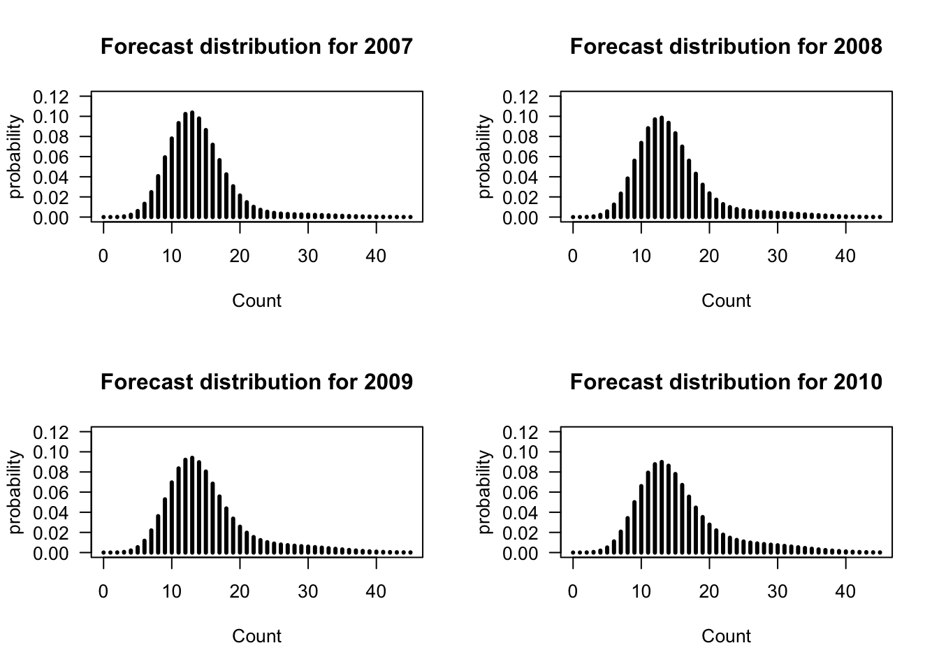
Figure 8.7: Forecast probabilities for the fitted three-state Poisson-HMM (non-stationary) for 1 to 4 years ahead.

The function from above can be modified to compute the bivariate forecast distribution.

pois.HMM.forecast_bivariate <- function(xf1, xf2, x, mod){
  n <- length(x)
  nxf1 <- length(xf1)
  nxf2 <- length(xf2)
  dxf <- matrix(0, nrow=nxf1, ncol=nxf2)
  foo <- mod$delta*dpois(x[1], mod$lambda)
  sumfoo <- sum(foo)
  lscale <- log(sumfoo)
  foo <- foo/sumfoo

  for(t in 2:n){
    foo <- foo%*%mod$gamma*dpois(x[t], mod$lambda)
    sumfoo <- sum(foo)
    lscale <- lscale + log(sumfoo)
    foo <- foo/sumfoo
  }

  for (i in 1:nxf1){
    for(j in 1:nxf2){
      for(s in 1:mod$m){
        dxf[i, j] <- dxf[i, j] + foo[s]*dpois(xf1[i], mod$lambda[s]) + foo[s]*dpois(xf2[j], mod$lambda[s])
      }
    }
  }

 return(foo)
}

For example, \(\Pr(X_{T+1} \leq 10, X_{T+2} \leq 10|\boldsymbol{X}^{(T)})\) is

eq_forecast <- data.frame(pois.HMM.forecast_bivariate(1:10, 1:10,eq_dat$Count, eq_init_ns))

eq_forecast %>%
  kbl(caption="Bivariate Forecast Distribution of $X_{T+1}$ (rows) and $X_{T+2}$ (columns).") %>%
  kable_minimal(full_width=T) %>%
  kable_styling()

Table 8.4: Bivariate Forecast Distribution of \(X_{T+1}\) (rows) and \(X_{T+2}\) (columns).

X1	X2	X3
0.961864	0.0370039	0.0011321

Decoding

Local decoding can be computed using the forward and backward algorithms from above. Similar to computing \(\hat{u}\) in the E step of the EM algorithm, the pois.HMM.state_probs computes the state probabilities then pois.HMM.local_decoding determines the most likely state at each time.

pois.HMM.state_probs <- function(x,mod)
{
 n          <- length(x)
 la         <- pois.HMM.lforward(x,mod)
 lb         <- pois.HMM.lbackward(x,mod)
 c          <- max(la[,n])
 llk        <- c+log(sum(exp(la[,n]-c)))
 stateprobs <- matrix(NA,ncol=n,nrow=mod$m)
 for (i in 1:n) stateprobs[,i]<-exp(la[,i]+lb[,i]-llk)
 return(stateprobs)
}

pois.HMM.local_decoding <- function(x,mod)
{
 n          <- length(x)
 stateprobs <- pois.HMM.state_probs(x,mod)
 ild        <- rep(NA,n)
 for (i in 1:n) ild[i]<-which.max(stateprobs[,i])
 ild
}

For example, local decoding for the three state Poisson-HMM (non-stationary) is

# Local decoding
(earthquake_local <- pois.HMM.local_decoding(eq_dat$Count, eq_init_ns))

##   [1] 1 1 1 1 1 3 3 3 3 3 3 3 3 3 3 2 2 2 2 1 1 1 1 2 2 2 2 2 2 2 2 2 2 2 2 2 2
##  [38] 3 3 3 3 3 3 3 3 3 3 3 3 3 3 3 2 2 2 2 2 3 1 2 2 2 2 2 2 2 2 2 3 3 3 3 2 2
##  [75] 2 2 2 2 2 2 2 1 1 1 1 1 1 1 1 1 2 2 1 1 1 2 2 2 2 2 2 2 2 2 1 1 1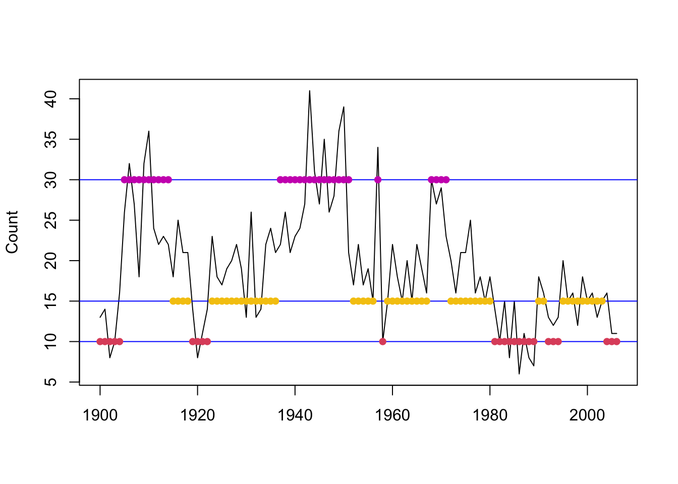

Figure 8.8: Local decoding for the three-state Poisson-HMM (non-stationary). The horizontal lines indicate the state-dependent means and the points indicate the decoded state at the given time.

We can also perform local decoding using momentuHMM

# Local decoding
## Compute state probabilities for each time step
state_probs <- stateProbs(mod3h_momentuHMM)

## Select state that maximizes probability
local_vec        <- rep(NA,length(eq_dat$Count))
for(i in 1:length(eq_dat$Count)) local_vec[i] <- which.max(state_probs[i,])
local_vec

##   [1] 1 1 1 1 1 3 3 3 3 3 3 3 2 2 2 2 2 2 2 1 1 1 1 2 2 2 2 2 2 2 2 2 2 2 2 2 2
##  [38] 2 2 2 2 3 3 3 3 3 3 3 3 3 3 2 2 2 2 2 2 2 2 2 2 2 2 2 2 2 2 2 3 3 3 2 2 2
##  [75] 2 2 2 2 2 2 1 1 1 1 1 1 1 1 1 1 1 1 1 1 1 1 1 1 1 1 1 1 1 1 1 1 1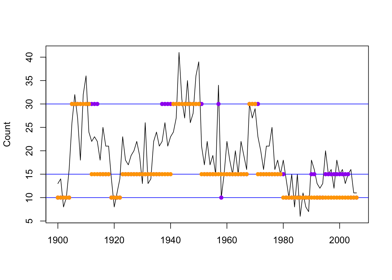

Figure 8.9: Local decoding for the three-state Poisson-HMM (non-stationary). The horizontal lines indicate the state-dependent means and the points indicate the decoded state at the given time using pois.HMM.local_decoding (purple) and momentuHMM (orange).

Global decoding can be computed using the Viterbi algorithm

pois.HMM.viterbi<-function(x,mod)
 {
 n              <- length(x)
 xi             <- matrix(0,n,mod$m)
 foo            <- mod$delta*dpois(x[1],mod$lambda)
 xi[1,]         <- foo/sum(foo)
 for (i in 2:n)
  {
  foo<-apply(xi[i-1,]*mod$gamma,2,max)*dpois(x[i],mod$lambda)
  xi[i,] <- foo/sum(foo)
  }
 iv<-numeric(n)
 iv[n]     <-which.max(xi[n,])
 for (i in (n-1):1)
   iv[i] <- which.max(mod$gamma[,iv[i+1]]*xi[i,])
 return(iv)
}

For example, global decoding for the three state Poisson-HMM (non-stationary) is

(earthquake_global <- pois.HMM.viterbi(eq_dat$Count, eq_init_ns))

##   [1] 1 1 1 1 1 3 3 3 3 3 3 3 3 3 3 3 3 3 3 1 1 1 1 2 2 2 2 2 2 2 2 2 2 2 2 2 2
##  [38] 2 3 3 3 3 3 3 3 3 3 3 3 3 3 2 2 2 2 2 2 2 2 2 2 2 2 2 2 2 2 2 3 3 3 3 2 2
##  [75] 2 2 2 2 2 2 2 1 1 1 1 1 1 1 1 1 1 1 1 1 1 2 2 2 2 2 2 2 2 2 2 1 1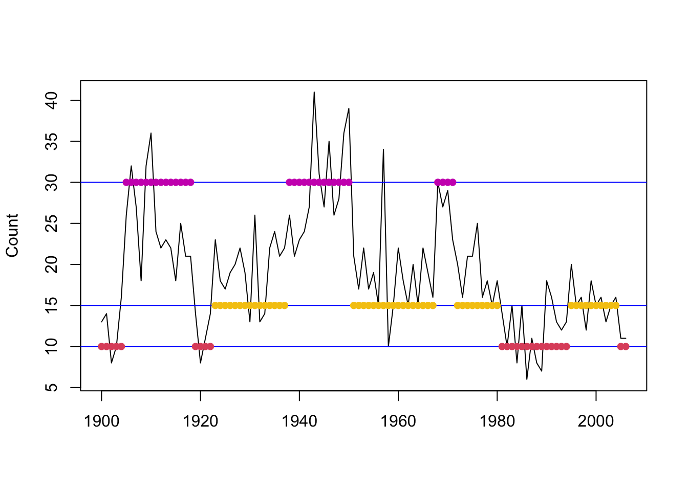

Figure 8.10: Global decoding for the three-state Poisson-HMM (non-stationary).

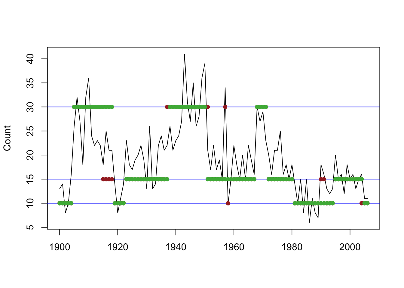
Figure 8.11: Global (green) and local (brown) decoding for the three-state Poisson-HMM (non-stationary).

The result of local and global decoding are very similar but not identical.

Similarly, we can perform global decoding using momentuHMM

(global_vec <- viterbi(mod3h_momentuHMM))

##   [1] 1 1 1 1 1 3 3 3 3 3 3 2 2 2 2 2 2 2 2 1 1 1 1 2 2 2 2 2 2 2 2 2 2 2 2 2 2
##  [38] 2 2 2 2 2 3 3 3 3 3 3 3 3 3 2 2 2 2 2 2 2 2 2 2 2 2 2 2 2 2 2 3 3 3 2 2 2
##  [75] 2 2 2 2 2 2 2 1 1 1 1 1 1 1 1 1 1 1 1 1 1 1 1 1 1 1 1 1 1 1 1 1 1

plotStates(mod3h_momentuHMM)

## Decoding state sequence... DONE
## Computing state probabilities... DONE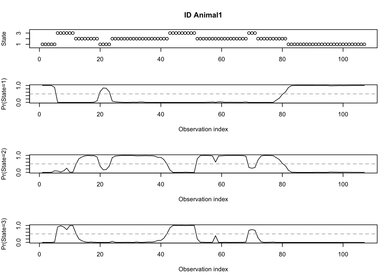

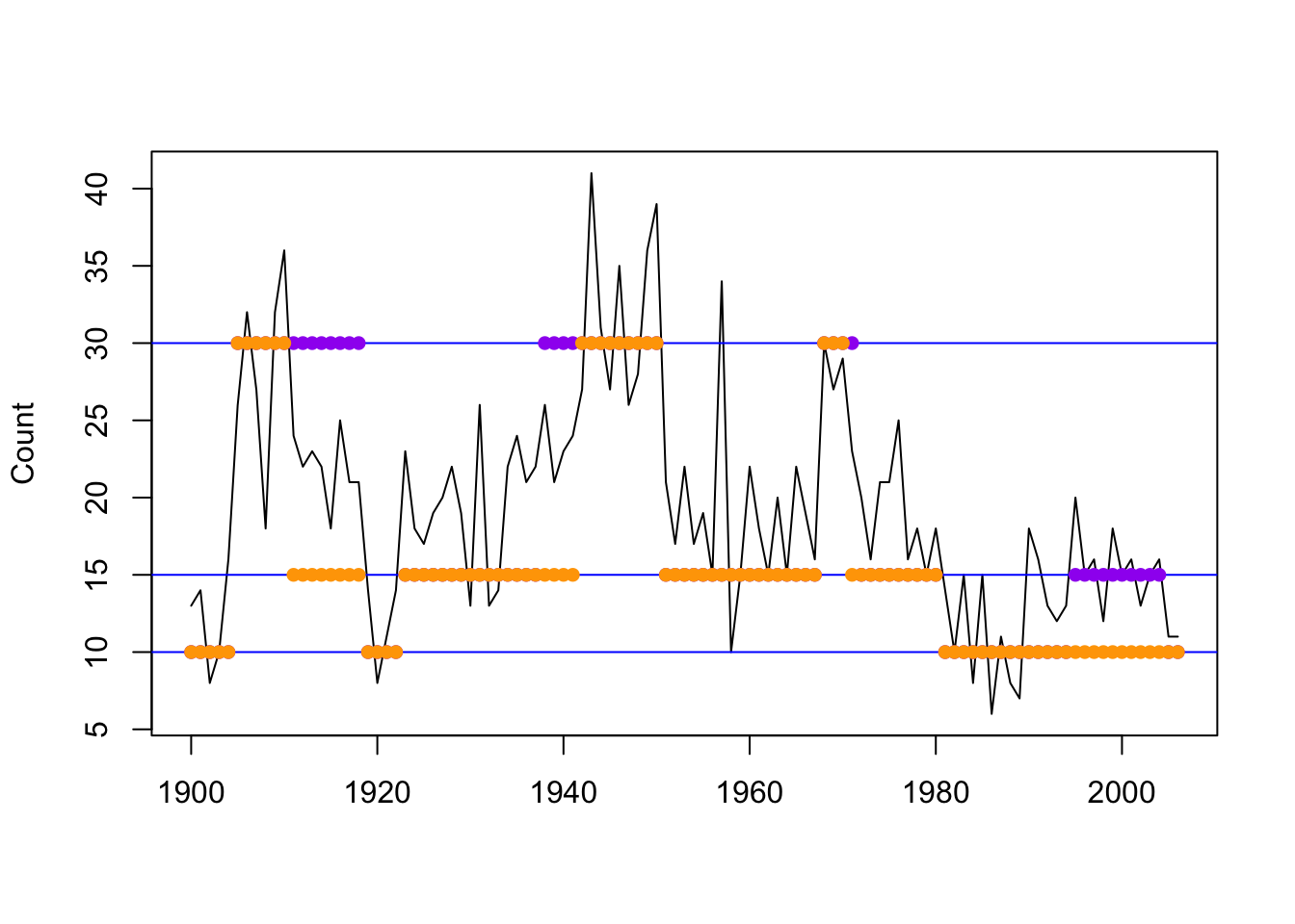
Figure 8.12: Global decoding for the three-state Poisson-HMM using pois.HMM.gocal_decoding (purple) and momentuHMM (orange).

There appears to be some differences between the results obtained from our function and from momentuHMM.

State Predictions

The state prediction for \(h\) steps ahead can be computed by

pois.HMM.state_prediction <- function(h=1,x,mod)
{
 n          <- length(x)
 la         <- pois.HMM.lforward(x,mod)
 c          <- max(la[,n])
 llk        <- c+log(sum(exp(la[,n]-c)))
 statepreds <- matrix(NA,ncol=h,nrow=mod$m)
 foo <- exp(la[,n]-llk)
 for (i in 1:h){
  foo<-foo%*%mod$gamma
  statepreds[,i]<-foo
  }
 return(statepreds)
}

For example, the state predictions for \(h=1, \dots, 5\) for the three-state Poisson-HMM (non-stationary)

pois.HMM.state_prediction(h=5, eq_dat$Count, eq_init_ns)

##           [,1]      [,2]      [,3]      [,4]      [,5]
## [1,] 0.7733048 0.6413134 0.5489194 0.4842436 0.4389705
## [2,] 0.1259027 0.1881319 0.2316923 0.2621846 0.2835292
## [3,] 0.1007924 0.1705547 0.2193883 0.2535718 0.2775003

The stationary distribution is

# Compute stationary distribution
solve(t(diag(m)-gamma+1),rep(1,m))

## [1] 0.3333333 0.3333333 0.3333333

Notice that as \(h \rightarrow \infty\), the state distribution approaches the stationary distribution.

Fitting a Poisson-HMM using STAN

Note: See Bayesian Inference for HMMs, Leos-Barajas and Michelot (2018), and Damiano, Peterson, and Weylandt (2017).

We can perform Bayesian inference for the three-state Poisson-HMM using STAN Stan Development Team (2023).

In STAN, the main building blocks are the:

data block: used to define the input data for the model to fit in STAN. Declare the data types, their dimensions, any restrictions, and their names of the data to model.

Here, we specify the length of the sequence of the earthquake series, the number of states, and the vector of observed earthquake counts.

'data{
int<lower=0> m;                       // number of states
int<lower=1> T;                       // length of sequence
int<lower=0> x[T];                    // observations
}
'

parameters block: used to define the parameters of the model that will be estimated. Declare the data types, their dimensions, any restrictions, and their names of the parameters to model.

Here, we specify the state-dependent means, transition probability matrix, and the initial distribution (assuming non-stationarity).

'parameters{
simplex[m] Gamma[m];                  // transition probability matrix
positive_ordered[m] lambda;           // state-dependent means (ordered to prevent label switching)
}

transformed parameters block: used to define any derived parameters that are not directly estimated but are derived from the parameters defined in the previous block. Declare the data types, their dimensions, any restrictions, their names, and the operation of the parameters to transform.

If we assume that the Markov Chain is stationary, then we can compute the stationary distribution from the tpm.

'transformed parameters{
  matrix[m, m] ta;                    // tpm used to compute stationary distribution                 
  simplex[m] statdist;                // stationary distribution

  for(j in 1:m){
    for(i in 1:m){
      ta[i, j] = Gamma[i, j];
    }
  }

//compute stationary distribution 
statdist =  to_vector((to_row_vector(rep_vector(1.0, m))/
      (diag_matrix(rep_vector(1.0, m)) - ta + rep_matrix(1, m, m))));
}
'

Note: The tpm is transposed so that each row corresponds to the probabilities of transitioning into a state, rather than out of a state.

model block: used to define the prior distribution, likelihood, and any other necessary variables.

Here, we use the following prior specifications:

\[\boldsymbol{\lambda} \sim Gamma(\alpha=1, \beta=0.01)\]

\[\boldsymbol{\Gamma} \sim Unif(-\infty, \infty)\]

\[\boldsymbol{\delta} \sim Unif(-\infty, \infty)\] The forward algorithm can be used to obtain the posterior distribution of the hidden states at a given time \(t\) based on all the information available up to that time \(\Pr(C_t|\boldsymbol{X}^{(t)})\).

\[\begin{align} \log (\alpha_t, j) &= \log \left(\sum_{i=1}^m \gamma_{ij} \alpha_{t-1, i} \right)\\ &= \log \left(\sum_{i=1}^m \exp (\log (\gamma_{ij}) + \log (\alpha_{t-1, i}))\right) \end{align}\]

'model{
  vector[m] log_Gamma_tr[m];
  vector[m] lp;
  vector[m] lp_p1;

  // priors
  lambda ~ gamma(1, 0.01);

  // transpose tpm and take log of entries
  for(i in 1:m)
    for(j in 1:m)
      log_Gamma_tr[j, i] = log(Gamma[i, j]);
    
  // forward algorithm
    // for t = 1
    for(i in 1:m)
      lp[i] = log(statdist[i]) + poisson_lpmf(x[1]|lambda[i]);
  
    // for t > 1
    for(t in 2:T){
      for (i in 1:m)
        lp_p1[i] = log_sum_exp(log_Gamma_tr[i] + lp) + poisson_lpmf(x[t]|lambda[i]);
      
        lp = lp_p1;
   }
   target += log_sum_exp(lp);
  }
'

## [1] "model{\n  vector[m] log_Gamma_tr[m];\n  vector[m] lp;\n  vector[m] lp_p1;\n\n  // priors\n  lambda ~ gamma(1, 0.01);\n\n  // transpose tpm and take log of entries\n  for(i in 1:m)\n    for(j in 1:m)\n      log_Gamma_tr[j, i] = log(Gamma[i, j]);\n    \n  // forward algorithm\n    // for t = 1\n    for(i in 1:m)\n      lp[i] = log(statdist[i]) + poisson_lpmf(x[1]|lambda[i]);\n  \n    // for t > 1\n    for(t in 2:T){\n      for (i in 1:m)\n        lp_p1[i] = log_sum_exp(log_Gamma_tr[i] + lp) + poisson_lpmf(x[t]|lambda[i]);\n      \n        lp = lp_p1;\n   }\n   target += log_sum_exp(lp);\n  }\n"

All together,

pois.HMM.stan <- 
'data{
int<lower=0> m;                       // number of states
int<lower=1> T;                       // length of sequence
int<lower=0> x[T];                    // observations
}

parameters{
simplex[m] Gamma[m];                  // tpm
positive_ordered[m] lambda;           // ordered mean of state-dependent (prevent label switching)
}

transformed parameters{
  matrix[m, m] ta;                    // tpm used to compute stationary distribution                 
  simplex[m] statdist;                // stationary distribution

  for(j in 1:m){
    for(i in 1:m){
      ta[i, j] = Gamma[i, j];
    }
  }

//compute stationary distribution 
statdist =  to_vector((to_row_vector(rep_vector(1.0, m))/
      (diag_matrix(rep_vector(1.0, m)) - ta + rep_matrix(1, m, m))));
}

model{
  // initialise
  vector[m] log_Gamma_tr[m];
  vector[m] lp;
  vector[m] lp_p1;

  // priors
  lambda ~ gamma(1, 0.01);

  // transpose tpm and take log of entries
  for(i in 1:m)
    for(j in 1:m)
      log_Gamma_tr[j, i] = log(Gamma[i, j]);
    
  // forward algorithm
  // for t = 1
  for(i in 1:m)
    lp[i] = log(statdist[i]) + poisson_lpmf(x[1]|lambda[i]);
  
  // loop over observations
  for(t in 2:T){
  // loop over states
    for (i in 1:m)
      lp_p1[i] = log_sum_exp(log_Gamma_tr[i] + lp) + poisson_lpmf(x[t]|lambda[i]);
      
      lp = lp_p1;
   }
   target += log_sum_exp(lp);
  }
'

Then for the three state-Poisson HMM,

# Format data into list for STAN
stan_data <- list(T=dim(eq_dat)[1], m=3, x=eq_dat$Count)

Running 2000 iterations for each of the 4 chains, with the first 1000 draws drawn during the warm-up phase,

pois.HMM.stanfit <- stan(model_code = pois.HMM.stan, data = stan_data, refresh=2000)

## Trying to compile a simple C file

## Running /Library/Frameworks/R.framework/Resources/bin/R CMD SHLIB foo.c
## clang -arch arm64 -I"/Library/Frameworks/R.framework/Resources/include" -DNDEBUG   -I"/Library/Frameworks/R.framework/Versions/4.2-arm64/Resources/library/Rcpp/include/"  -I"/Library/Frameworks/R.framework/Versions/4.2-arm64/Resources/library/RcppEigen/include/"  -I"/Library/Frameworks/R.framework/Versions/4.2-arm64/Resources/library/RcppEigen/include/unsupported"  -I"/Library/Frameworks/R.framework/Versions/4.2-arm64/Resources/library/BH/include" -I"/Library/Frameworks/R.framework/Versions/4.2-arm64/Resources/library/StanHeaders/include/src/"  -I"/Library/Frameworks/R.framework/Versions/4.2-arm64/Resources/library/StanHeaders/include/"  -I"/Library/Frameworks/R.framework/Versions/4.2-arm64/Resources/library/RcppParallel/include/"  -I"/Library/Frameworks/R.framework/Versions/4.2-arm64/Resources/library/rstan/include" -DEIGEN_NO_DEBUG  -DBOOST_DISABLE_ASSERTS  -DBOOST_PENDING_INTEGER_LOG2_HPP  -DSTAN_THREADS  -DBOOST_NO_AUTO_PTR  -include '/Library/Frameworks/R.framework/Versions/4.2-arm64/Resources/library/StanHeaders/include/stan/math/prim/mat/fun/Eigen.hpp'  -D_REENTRANT -DRCPP_PARALLEL_USE_TBB=1   -I/opt/R/arm64/include   -fPIC  -falign-functions=64 -Wall -g -O2  -c foo.c -o foo.o
## In file included from <built-in>:1:
## In file included from /Library/Frameworks/R.framework/Versions/4.2-arm64/Resources/library/StanHeaders/include/stan/math/prim/mat/fun/Eigen.hpp:13:
## In file included from /Library/Frameworks/R.framework/Versions/4.2-arm64/Resources/library/RcppEigen/include/Eigen/Dense:1:
## In file included from /Library/Frameworks/R.framework/Versions/4.2-arm64/Resources/library/RcppEigen/include/Eigen/Core:88:
## /Library/Frameworks/R.framework/Versions/4.2-arm64/Resources/library/RcppEigen/include/Eigen/src/Core/util/Macros.h:628:1: error: unknown type name 'namespace'
## namespace Eigen {
## ^
## /Library/Frameworks/R.framework/Versions/4.2-arm64/Resources/library/RcppEigen/include/Eigen/src/Core/util/Macros.h:628:16: error: expected ';' after top level declarator
## namespace Eigen {
##                ^
##                ;
## In file included from <built-in>:1:
## In file included from /Library/Frameworks/R.framework/Versions/4.2-arm64/Resources/library/StanHeaders/include/stan/math/prim/mat/fun/Eigen.hpp:13:
## In file included from /Library/Frameworks/R.framework/Versions/4.2-arm64/Resources/library/RcppEigen/include/Eigen/Dense:1:
## /Library/Frameworks/R.framework/Versions/4.2-arm64/Resources/library/RcppEigen/include/Eigen/Core:96:10: fatal error: 'complex' file not found
## #include <complex>
##          ^~~~~~~~~
## 3 errors generated.
## make: *** [foo.o] Error 1
## 
## SAMPLING FOR MODEL '9875485ac4343cdf02f82dbe9761d256' NOW (CHAIN 1).
## Chain 1: 
## Chain 1: Gradient evaluation took 0.000123 seconds
## Chain 1: 1000 transitions using 10 leapfrog steps per transition would take 1.23 seconds.
## Chain 1: Adjust your expectations accordingly!
## Chain 1: 
## Chain 1: 
## Chain 1: Iteration:    1 / 2000 [  0%]  (Warmup)
## Chain 1: Iteration: 1001 / 2000 [ 50%]  (Sampling)
## Chain 1: Iteration: 2000 / 2000 [100%]  (Sampling)
## Chain 1: 
## Chain 1:  Elapsed Time: 0.820039 seconds (Warm-up)
## Chain 1:                0.450072 seconds (Sampling)
## Chain 1:                1.27011 seconds (Total)
## Chain 1: 
## 
## SAMPLING FOR MODEL '9875485ac4343cdf02f82dbe9761d256' NOW (CHAIN 2).
## Chain 2: 
## Chain 2: Gradient evaluation took 5e-05 seconds
## Chain 2: 1000 transitions using 10 leapfrog steps per transition would take 0.5 seconds.
## Chain 2: Adjust your expectations accordingly!
## Chain 2: 
## Chain 2: 
## Chain 2: Iteration:    1 / 2000 [  0%]  (Warmup)
## Chain 2: Iteration: 1001 / 2000 [ 50%]  (Sampling)
## Chain 2: Iteration: 2000 / 2000 [100%]  (Sampling)
## Chain 2: 
## Chain 2:  Elapsed Time: 0.823041 seconds (Warm-up)
## Chain 2:                0.527402 seconds (Sampling)
## Chain 2:                1.35044 seconds (Total)
## Chain 2: 
## 
## SAMPLING FOR MODEL '9875485ac4343cdf02f82dbe9761d256' NOW (CHAIN 3).
## Chain 3: 
## Chain 3: Gradient evaluation took 4.9e-05 seconds
## Chain 3: 1000 transitions using 10 leapfrog steps per transition would take 0.49 seconds.
## Chain 3: Adjust your expectations accordingly!
## Chain 3: 
## Chain 3: 
## Chain 3: Iteration:    1 / 2000 [  0%]  (Warmup)
## Chain 3: Iteration: 1001 / 2000 [ 50%]  (Sampling)
## Chain 3: Iteration: 2000 / 2000 [100%]  (Sampling)
## Chain 3: 
## Chain 3:  Elapsed Time: 0.812108 seconds (Warm-up)
## Chain 3:                0.457366 seconds (Sampling)
## Chain 3:                1.26947 seconds (Total)
## Chain 3: 
## 
## SAMPLING FOR MODEL '9875485ac4343cdf02f82dbe9761d256' NOW (CHAIN 4).
## Chain 4: 
## Chain 4: Gradient evaluation took 4.9e-05 seconds
## Chain 4: 1000 transitions using 10 leapfrog steps per transition would take 0.49 seconds.
## Chain 4: Adjust your expectations accordingly!
## Chain 4: 
## Chain 4: 
## Chain 4: Iteration:    1 / 2000 [  0%]  (Warmup)
## Chain 4: Iteration: 1001 / 2000 [ 50%]  (Sampling)
## Chain 4: Iteration: 2000 / 2000 [100%]  (Sampling)
## Chain 4: 
## Chain 4:  Elapsed Time: 0.76585 seconds (Warm-up)
## Chain 4:                0.455552 seconds (Sampling)
## Chain 4:                1.2214 seconds (Total)
## Chain 4:

we obtain the following posterior estimates

print(pois.HMM.stanfit,digits_summary = 3)

## Inference for Stan model: 9875485ac4343cdf02f82dbe9761d256.
## 4 chains, each with iter=2000; warmup=1000; thin=1; 
## post-warmup draws per chain=1000, total post-warmup draws=4000.
## 
##                 mean se_mean    sd     2.5%      25%      50%      75%    97.5%
## Gamma[1,1]     0.862   0.002 0.085    0.669    0.825    0.879    0.919    0.966
## Gamma[1,2]     0.091   0.002 0.076    0.006    0.039    0.073    0.122    0.274
## Gamma[1,3]     0.047   0.001 0.042    0.002    0.017    0.036    0.066    0.152
## Gamma[2,1]     0.090   0.002 0.065    0.014    0.048    0.077    0.115    0.237
## Gamma[2,2]     0.817   0.002 0.085    0.626    0.778    0.831    0.874    0.935
## Gamma[2,3]     0.093   0.001 0.058    0.015    0.051    0.083    0.120    0.237
## Gamma[3,1]     0.077   0.001 0.069    0.002    0.025    0.059    0.110    0.249
## Gamma[3,2]     0.231   0.002 0.115    0.055    0.148    0.214    0.300    0.493
## Gamma[3,3]     0.691   0.002 0.124    0.423    0.609    0.706    0.783    0.891
## lambda[1]     13.198   0.019 0.857   11.423   12.686   13.221   13.729   14.875
## lambda[2]     19.828   0.026 1.069   17.689   19.181   19.836   20.478   21.929
## lambda[3]     29.905   0.036 1.905   26.419   28.600   29.855   31.105   33.882
## ta[1,1]        0.862   0.002 0.085    0.669    0.825    0.879    0.919    0.966
## ta[1,2]        0.091   0.002 0.076    0.006    0.039    0.073    0.122    0.274
## ta[1,3]        0.047   0.001 0.042    0.002    0.017    0.036    0.066    0.152
## ta[2,1]        0.090   0.002 0.065    0.014    0.048    0.077    0.115    0.237
## ta[2,2]        0.817   0.002 0.085    0.626    0.778    0.831    0.874    0.935
## ta[2,3]        0.093   0.001 0.058    0.015    0.051    0.083    0.120    0.237
## ta[3,1]        0.077   0.001 0.069    0.002    0.025    0.059    0.110    0.249
## ta[3,2]        0.231   0.002 0.115    0.055    0.148    0.214    0.300    0.493
## ta[3,3]        0.691   0.002 0.124    0.423    0.609    0.706    0.783    0.891
## statdist[1]    0.391   0.002 0.142    0.143    0.286    0.380    0.485    0.688
## statdist[2]    0.418   0.002 0.130    0.172    0.326    0.416    0.509    0.679
## statdist[3]    0.191   0.001 0.092    0.056    0.124    0.177    0.240    0.414
## lp__        -345.917   0.079 2.515 -351.814 -347.287 -345.502 -344.077 -342.235
##             n_eff  Rhat
## Gamma[1,1]   2066 1.000
## Gamma[1,2]   1987 1.000
## Gamma[1,3]   4086 1.001
## Gamma[2,1]   1333 1.002
## Gamma[2,2]   1526 1.002
## Gamma[2,3]   3405 1.000
## Gamma[3,1]   3718 1.001
## Gamma[3,2]   4353 1.000
## Gamma[3,3]   3762 1.001
## lambda[1]    1953 1.002
## lambda[2]    1658 1.000
## lambda[3]    2877 1.001
## ta[1,1]      2066 1.000
## ta[1,2]      1987 1.000
## ta[1,3]      4086 1.001
## ta[2,1]      1333 1.002
## ta[2,2]      1526 1.002
## ta[2,3]      3405 1.000
## ta[3,1]      3718 1.001
## ta[3,2]      4353 1.000
## ta[3,3]      3762 1.001
## statdist[1]  5011 1.000
## statdist[2]  3710 1.001
## statdist[3]  4474 1.001
## lp__         1025 1.004
## 
## Samples were drawn using NUTS(diag_e) at Fri Jun 16 13:19:35 2023.
## For each parameter, n_eff is a crude measure of effective sample size,
## and Rhat is the potential scale reduction factor on split chains (at 
## convergence, Rhat=1).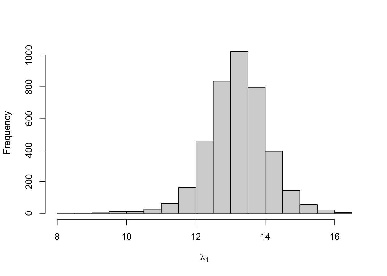

Figure 8.13: Posterior distribution for the state-dependent means of the three-state Poisson-HMM.

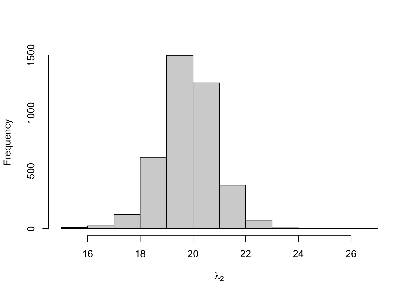
Figure 8.14: Posterior distribution for the state-dependent means of the three-state Poisson-HMM.

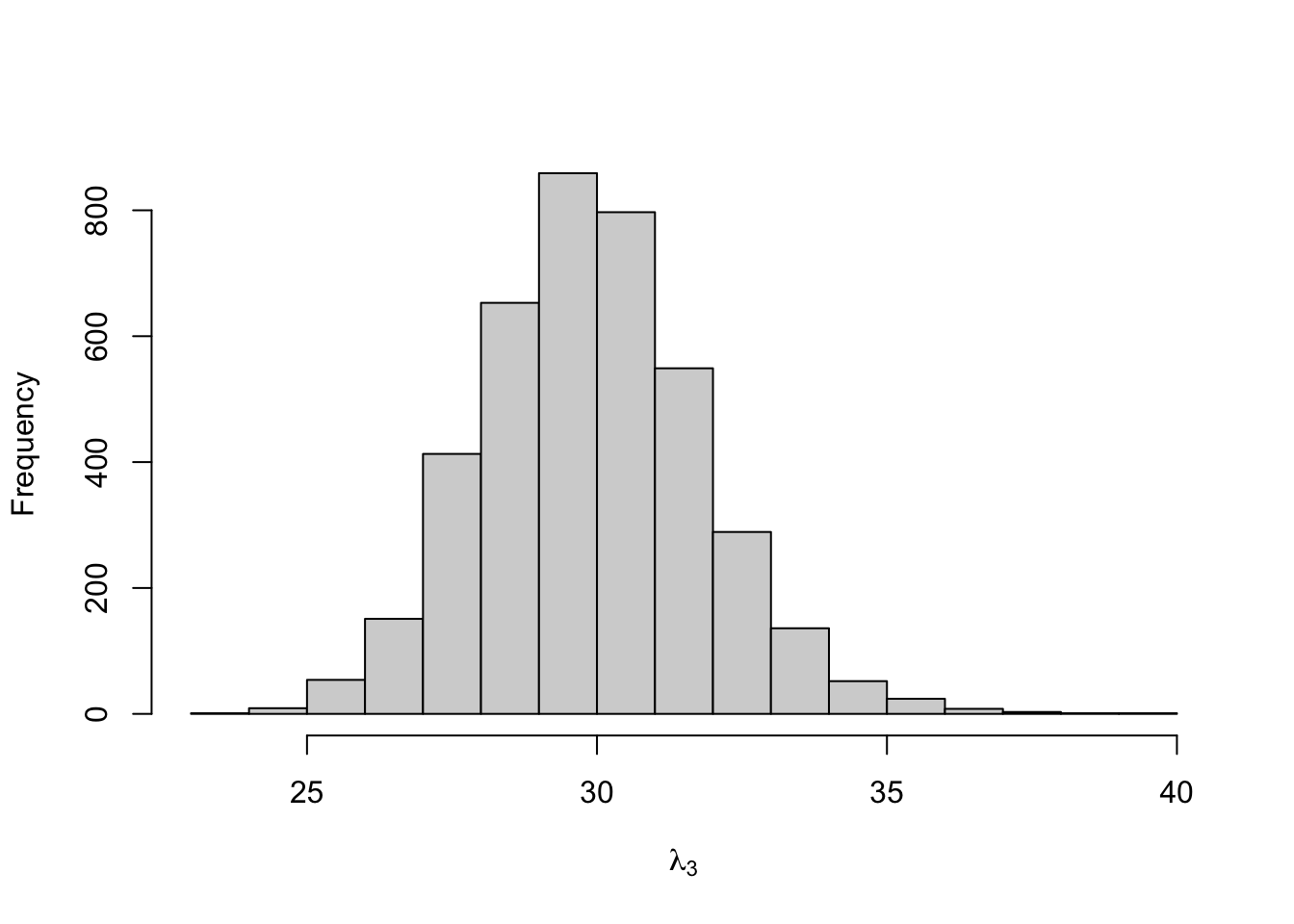
Figure 8.15: Posterior distribution for the state-dependent means of the three-state Poisson-HMM.

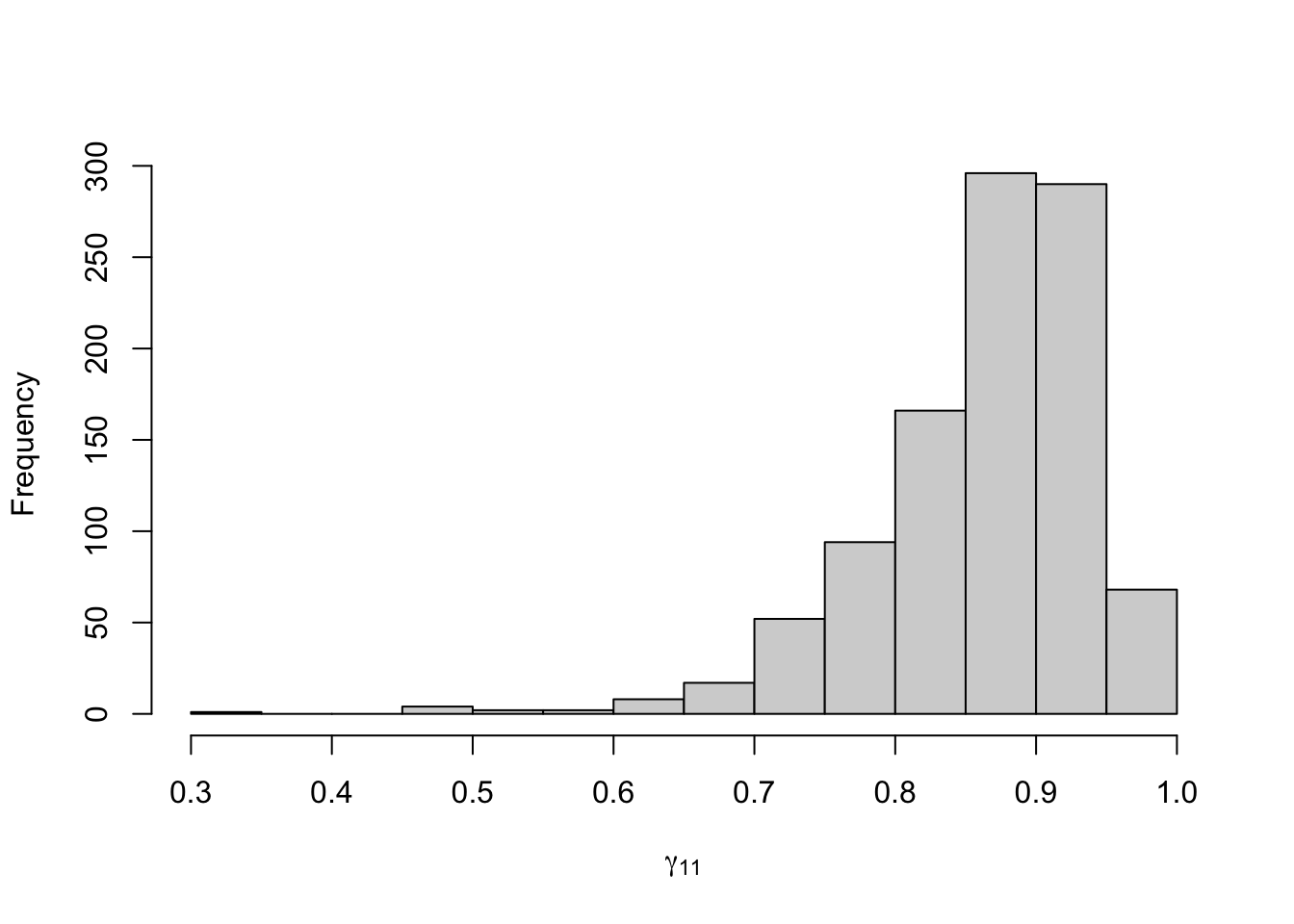
Figure 8.16: Posterior distribution for the transition probabilities of the three-state Poisson-HMM.

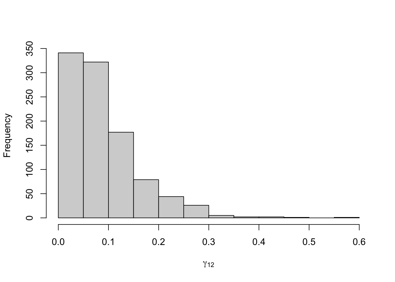
Figure 8.17: Posterior distribution for the transition probabilities of the three-state Poisson-HMM.

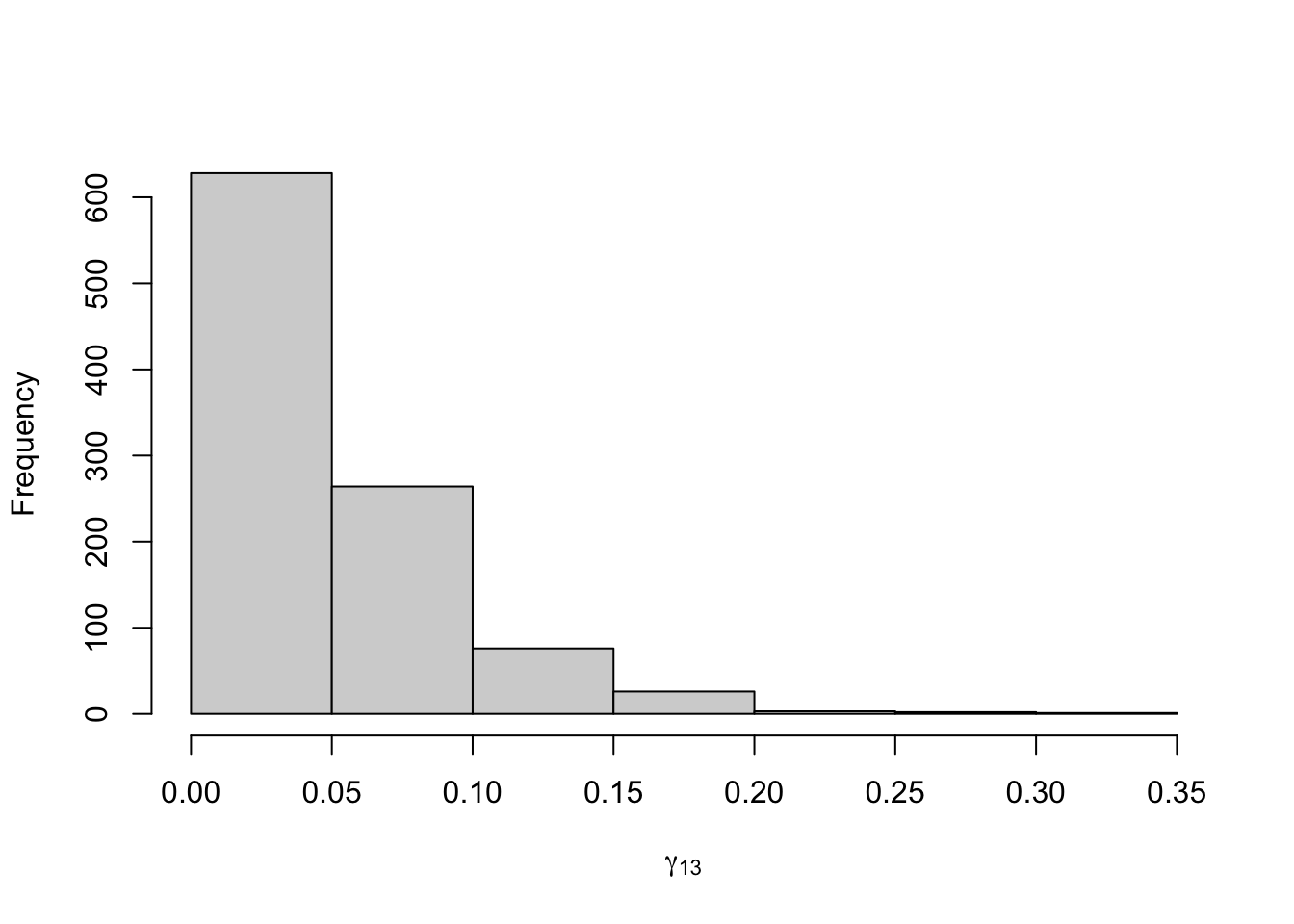
Figure 8.18: Posterior distribution for the transition probabilities of the three-state Poisson-HMM.

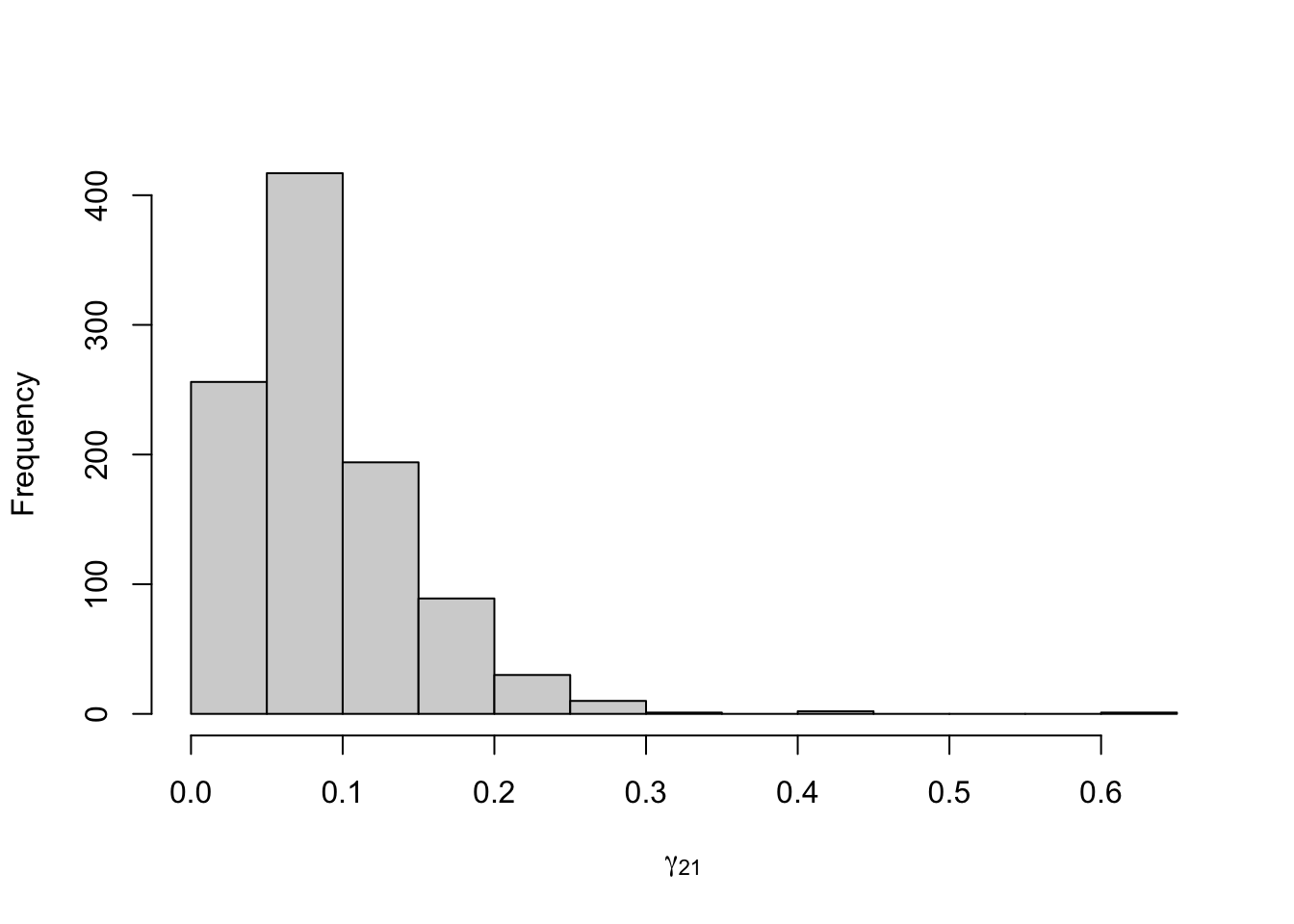
Figure 8.19: Posterior distribution for the transition probabilities of the three-state Poisson-HMM.

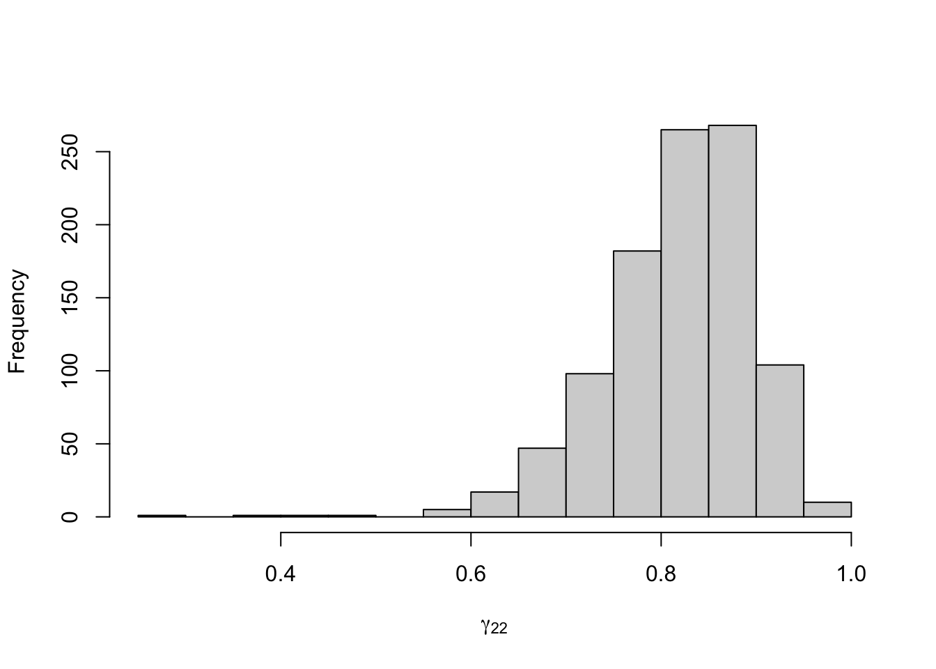
Figure 8.20: Posterior distribution for the transition probabilities of the three-state Poisson-HMM.

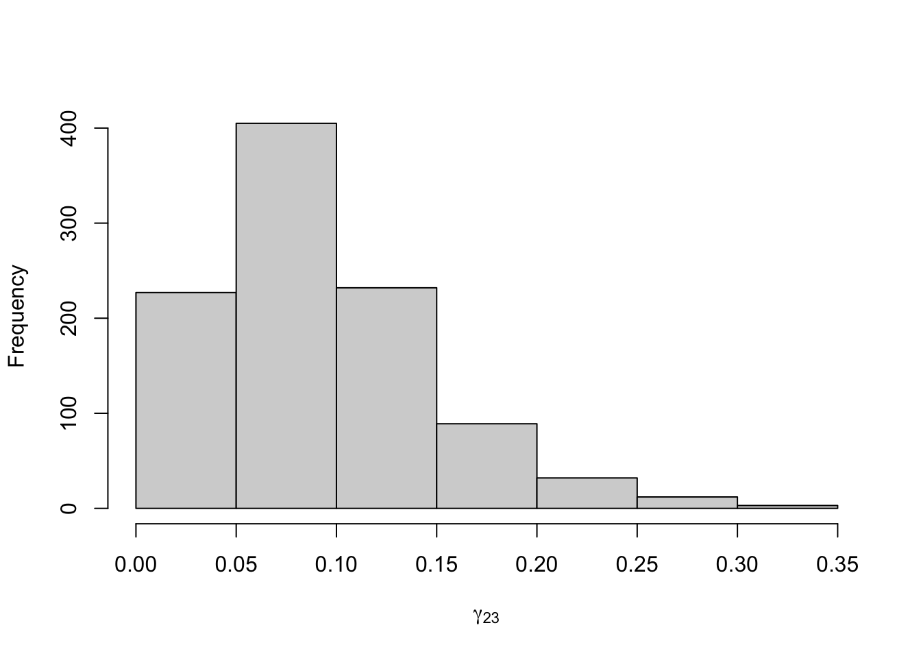
Figure 8.21: Posterior distribution for the transition probabilities of the three-state Poisson-HMM.

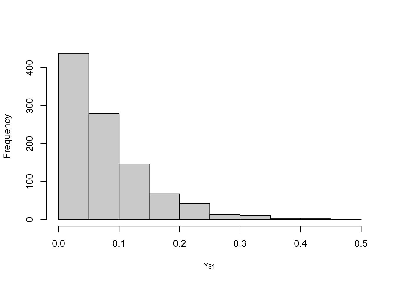
Figure 8.22: Posterior distribution for the transition probabilities of the three-state Poisson-HMM.

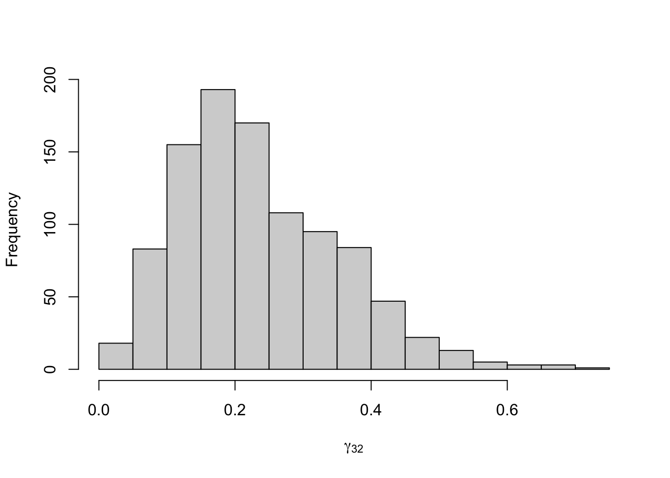
Figure 8.23: Posterior distribution for the transition probabilities of the three-state Poisson-HMM.

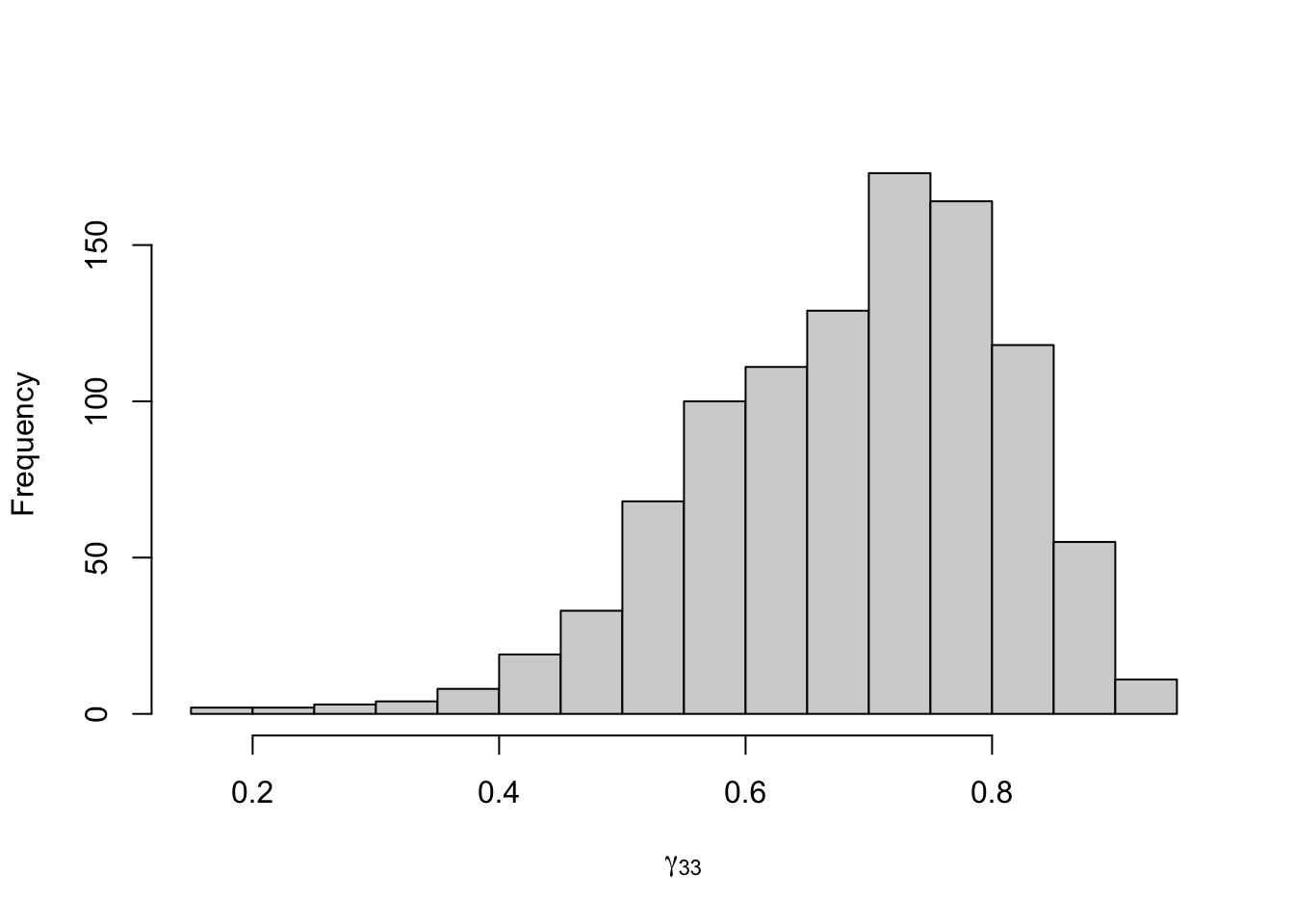
Figure 8.24: Posterior distribution for the transition probabilities of the three-state Poisson-HMM.

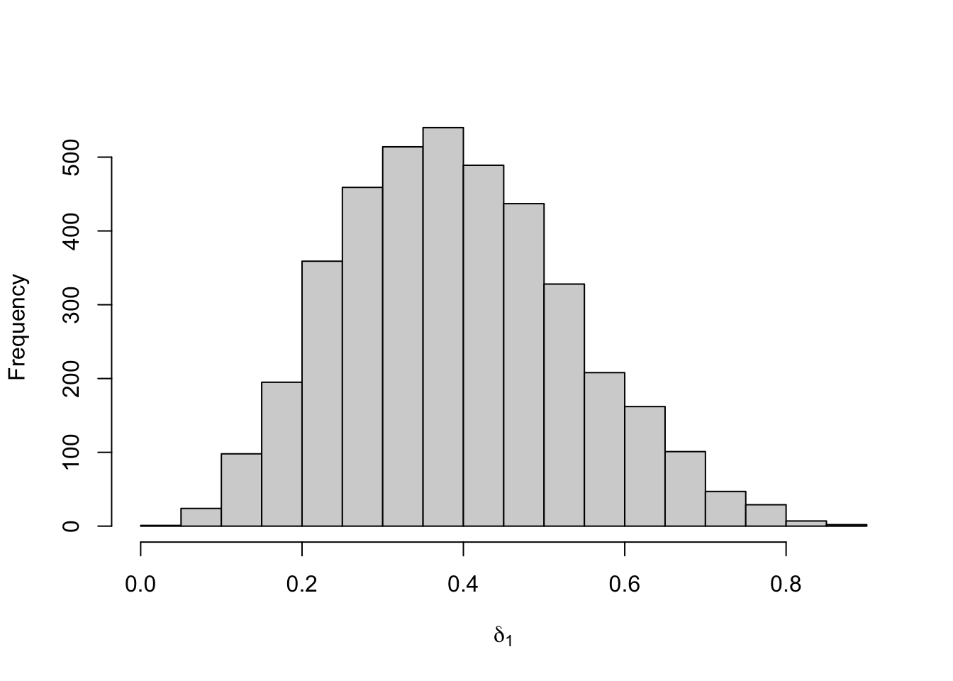
Figure 8.25: Posterior distribution for the initial distribution of the three-state Poisson-HMM.

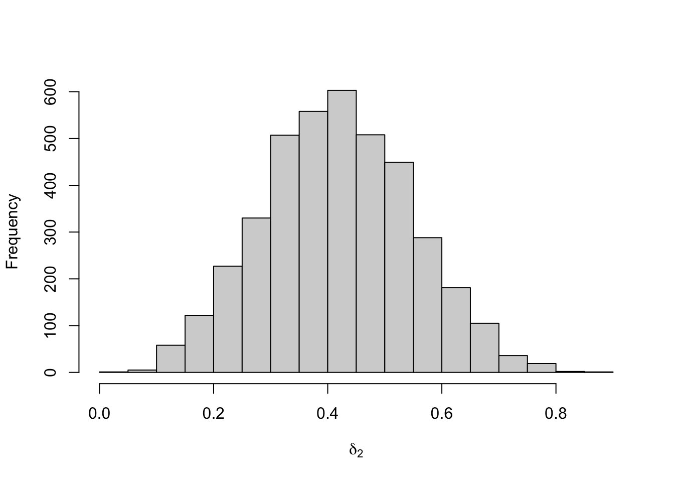
Figure 8.26: Posterior distribution for the initial distribution of the three-state Poisson-HMM.

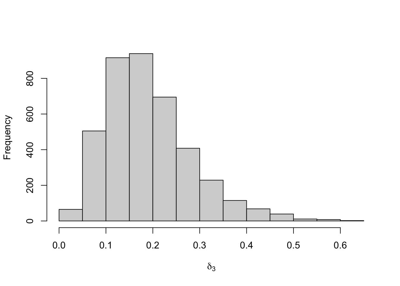
Figure 8.27: Posterior distribution for the initial distribution of the three-state Poisson-HMM.

References

Damiano, Luis, Brian Peterson, and Michael Weylandt. 2017. A Tutorial on Hidden Markov Models Using Stan. https://luisdamiano.github.io/stancon18/hmm_stan_tutorial.pdf.

Leos-Barajas, Vianey, and Théo Michelot. 2018. “An Introduction to Animal Movement Modeling with Hidden Markov Models Using Stan for Bayesian Inference.” https://arxiv.org/abs/1806.10639.

McClintock, Brett T., and Th’eo Michelot. 2018. “MomentuHMM: R Package for Generalized Hidden Markov Models of Animal Movement.” Methods in Ecology and Evolution 9 (6): 1518–30. https://doi.org/10.1111/2041-210X.12995.

Stan Development Team. 2023. “RStan: The R Interface to Stan.” https://mc-stan.org/.